Recurrent Predictive Routing: Learning What to Remember, Predict, and Follow
Revision 2 · Single-layer design under review. This article separates a concrete, dimensioned implementation sketch from the research questions it leaves open. The diagrams run scripted geometry, not trained RPR. There are no experimental results yet.
The problem: the world does not arrive as a sequence of independent frames
A robot sees a room, turns its camera, moves an arm, feels contact, and senses the consequences. Useful information lives both in individual observations and in how they change together:
- Which earlier signals help predict the next signal?
- Which relationships deserve computation now?
- Which observations belong to the same continuing thing?
- How can actions gather evidence that distinguishes competing explanations?
The first two questions concern predictive routing. The third concerns correspondence: deciding that observations at different times, locations, or sensors refer to the same entity. The fourth connects both to active sensing.
Recurrent Predictive Routing (RPR) explores a sparse network of learned predictive relationships. Its central unfinished question is how to organize those relationships into coherent, persistent explanations of the world. Accurate local prediction does not establish object identity.
A layman’s picture
Imagine watching a basketball, then lowering your camera toward a black line on the court. Orange pixels on the ball help predict nearby orange pixels; its black seams help predict nearby black pixels. After the camera moves, the court line also produces easy-to-predict black pixels.
A system could predict this entire sequence reasonably well while mixing evidence about the ball and the floor into the same memory. “I correctly predicted another black pixel” does not tell it which thing that pixel belongs to.
RPR therefore needs two kinds of progress: learning useful temporal relationships, and discovering where their evidence should accumulate. The first has a concrete working sketch below. The second is reserved for an interactive design session near the end.
Architecture at a glance
A token is one indexed unit of input presented to this layer. In our small example it is a sensor channel’s recent samples. A node is the processing/state record associated with that token.
A relationship pair is an ordered index pair (i, j): use evidence from input i to help predict input j. A route is the gate attached to that pair. The pair identifies the relationship; the gate decides whether its predictive contribution is computed or passed onward. In a graph drawing, that selected relationship is a directed graph edge.
Here is the complete single-layer roadmap. The numbers 1–5 match the explanation below. Stages 1a–1d are deliberately expanded: encoding, learned expansion, and recurrent calculation all happen before the compatibility matrix.
h names the short-history encoding; n names its expanded learned representation; s names recurrent per-token state; e names recurrent pair state. They are separate quantities in this revision.
flowchart TD
    X[/"Sensor samples and applied action"/] --> B["1a · Per-index four-sample buffers"]
    B --> H["1b · Encode each buffer: h"]
    H --> N["1c · Learned expansion: n"]
    N --> S["1d · Recurrent encoder: s"]
    S --> D[("Store s until next tick")]
    D --> S
    S --> C["2 · Compatibility matrix C"]
    C --> G{"2 · Select pair gates"}
    G --> E["3 · Update selected pair states e"]
    N --> E
    E --> ED[("Store pair state and age")]
    ED --> E
    E --> M["4 · Decode and combine predictions"]
    N --> M
    S --> M
    M --> P[("Cache forecasts made at this tick")]
    P --> L["5 · Score when the next sample arrives"]
    X --> L
    L -. training and later gate statistics .-> C
Buffers are drawn as sample storage, cylinders as state retained across ticks, a diamond as gate selection, and rectangles as computations. The detailed figures below open those computations into history cells, feature vectors, a feedback loop, and a matrix.
The fixed widths and GRUs below are proposed implementation choices, not established properties of RPR. The previous draft used n for a GRU state; this revision reserves n for the learned expanded encoding and gives the recurrent state its own symbol, s. That makes the distinction explicit rather than letting one symbol change meaning mid-explanation.
The working scope is one layer. A later hierarchy would reuse this kind of transformation on different inputs and separately maintained states; whether weights should be shared is a separate design choice.
A concrete toy world
Consider a camera at position \((0.5,1.5)\text{ m}\) in a \(4\text{ m}\times3\text{ m}\) room. A green marker sits at \((2.8,2.1)\text{ m}\), and an amber marker at \((3.2,0.8)\text{ m}\). Counterclockwise angles are positive. The green marker’s initial bearing is about \(+14.62^\circ\), at range \(2.38\text{ m}\).
The camera’s illustrative 110-degree field of view has twelve soft sampling locations:
\[b_i=-55^\circ+10^\circ i,\qquad i=0,\ldots,11.\]bin_centers_degrees = [-55, -45, -35, -25, -15, -5,
5, 15, 25, 35, 45, 55]
To avoid handing object identity to the learner, the revised input sketch combines the two markers into one scalar intensity per visual bin. The green/amber labels are available to the illustration and evaluation code, not as separate “target” and “distractor” input channels.
| Token index | Meaning | One sample at time t |
|---|---|---|
| 0–11 | Visual bins, ordered from −55° to +55° | Combined scalar intensity |
| 12 | Camera orientation, first component | sin(pan angle) |
| 13 | Camera orientation, second component | cos(pan angle) |
| 14 | Pan command committed at this tick for the next interval | Angular velocity, divided by a chosen scale |
Thus there are 15 indexed scalar streams, not fifteen known objects. Tokens 12 and 13 together describe one physical angle; splitting them is an explicit input-design choice. The command is an exogenous input: the model receives it but is not rewarded for guessing the next externally selected command.
Interactive world and sensor geometry
Move the slider to step through six scripted camera positions. The world panel shows physical locations; the sensor panel shows how the same geometry changes the sampled intensities.
What runs behind the diagram? The site’s JavaScript file, rpr-visualizer.js, uses Plotly to render a fixed sequence at times 0.0–0.5 seconds. The pan angles are manually specified as [0, 3, 6, 9, 12, 14] degrees. Commands [30, 30, 30, 30, 20, 0] degrees/second are the outgoing commands for those frames; the first five integrate to the next angle with a 0.1-second interval. The external controller commits the outgoing command before the predictor runs, so channel 14 supplies that known action alongside the current measurements. This timing makes the forecast action-conditioned without exposing future measurements.
For marker \(o\), the program calculates its bearing relative to the camera and a Gaussian response at each bin. The scalar input is the clipped sum:
\[\begin{aligned} \beta_o[t]&=\operatorname{atan2}(y_o-y_c,x_o-x_c)-\phi[t],\\ A_{io}[t]&=\exp\left(-\frac{(b_i-\beta_o[t])^2}{2\sigma^2}\right),\\ x_i[t]&=\min\left(1,\sum_o A_{io}[t]\right),\qquad \sigma=6^\circ . \end{aligned}\]bearing = degrees(atan2(marker.y - camera.y, marker.x - camera.x))
relative_bearing = bearing - pan_degrees
response[bin, marker] = (
exp(-0.5 * ((bin_degrees - relative_bearing) / 6)**2)
if abs(relative_bearing) <= 55 else 0
)
sensor_input[bin] = min(1, sum(response[bin, marker] for marker in markers))
All angular quantities must use consistent units in the Gaussian calculation; the code converts atan2 to degrees. Colored response components are diagnostic overlays; the combined bars are the proposed visual inputs. Responses outside the field of view are suppressed.
This is a scripted sensor-geometry illustration. It runs neither an RPR network nor a feedback controller or trained reference baseline. It demonstrates the input transformation a predictor would have to learn. It provides no evidence of learned tracking.
The 3D view uses the same scripted values as coordinates. Its axes are physical quantities, not learned latent dimensions.
1. From sensor samples to an expanded recurrent representation
The first stage runs independently for each sensor index. The diagram shows one such lane; there are fifteen lanes with separate buffers and recurrent states.
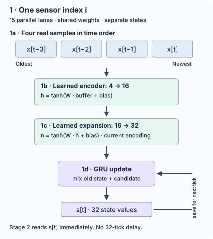
1a — Buffer the input. For each index \(i\), collect the last four scalar samples:
\[B_i[t]=[x_i[t-3],x_i[t-2],x_i[t-1],x_i[t]]\in\mathbb R^4.\]for i in 0..14:
buffer[i] = last_four_samples_of_stream(i) # [4]
# Whole batch: [15, 4]. Begin forecasting after four real samples.
This buffer is a literal short shift register. At 10 Hz it spans 0.3 seconds from oldest to newest sample. Normalize each channel with fixed training-set scales. A practical stream must additionally specify missing-sample handling and timestamps.
1b — Encode that short pattern. A learned feed-forward encoder expands four samples into sixteen features:
\[h_i[t]=\tanh(W_h B_i[t]+b_h),\qquad W_h\in\mathbb R^{16\times4}.\]h[i] = tanh(linear_4_to_16(buffer[i])) # [16]
Sixteen is a chosen feature width, not sixteen timestamps. The encoder can form combinations of level, change, curvature, and other patterns from the four samples. It does not create new observations. The same encoder weights can be shared across normalized channels while each index keeps its own data.
1c — Expand the learned representation. A second learned encoder produces the 32-value representation called \(n_i[t]\):
\[n_i[t]=\tanh(W_n h_i[t]+b_n),\qquad W_n\in\mathbb R^{32\times16}.\]n[i] = tanh(linear_16_to_32(h[i])) # [32], recomputed this tick
Here n is an expanded description of the recent sensor pattern, produced by its own learned projection. It is used both to form recurrent context and to update the pairwise relationship model in stage 3. Width 32 is another tunable capacity choice, not an additional 32 samples or a guarantee of richer information.
1d — Integrate with previous recurrent state. A GRU (gated recurrent unit) takes this tick’s 32-value encoding and the previous 32-value state to produce \(s_i[t]\):
\[s_i[t]=\operatorname{GRU}_{\rm local}(n_i[t],s_i[t-1]) \in\mathbb R^{32}.\]s[i] = local_gru(input=n[i], previous_state=s_prev[i]) # [32]
# All 15 lanes update; stage 2 then receives s with shape [15, 32].
A GRU uses learned gates to mix a candidate state with retained previous state. One conventional parameterization is:
\[\begin{aligned} z&=\sigma(W_z n+U_z s_{\rm old}+b_z),\\ r&=\sigma(W_r n+U_r s_{\rm old}+b_r),\\ \widetilde{s}&=\tanh(W_s n+U_s(r\odot s_{\rm old})+b_s),\\ s_{\rm new}&=(1-z)\odot s_{\rm old}+z\odot\widetilde{s}. \end{aligned}\]update_gate = sigmoid(input_projection(n) + state_projection(old_state))
reset_gate = sigmoid(other_input_projection(n) + other_state_projection(old_state))
candidate = tanh(candidate_input(n) + candidate_state(reset_gate * old_state))
new_state = (1 - update_gate) * old_state + update_gate * candidate
Each gate has 32 components; * in the last two lines is elementwise multiplication. The matrices are learned, with separate weights for each named projection. Gate conventions differ between implementations; this is one explicit convention.
The GRU returns the current state immediately at every tick. An unrolled drawing shows repeated calls to the same cell across time, with shared weights. It is not a pipeline that waits for the sample to travel through 32 delayed stages. Only the four-sample buffer literally shifts samples.
What teaches these encoders? A prediction head reads s to forecast the next raw normalized sensor value. The next actual sample supplies the error, which trains the head, GRU, and n/h encoders together through backpropagation through time. Pairwise losses provide additional training signal in stages 3–5. No individual latent coordinate is preassigned “confidence” or “object identity.” Predicting raw measurements also avoids an unconstrained learned-target collapse in which both a latent target and its forecast become constant.
The input-to-state pipeline is now complete: four samples → 16 features → 32 expanded features → 32 recurrent-state values, per index.
2. Compatibility becomes a matrix of pair gates
Now place the fifteen current recurrent vectors into a matrix \(S[t]\in\mathbb R^{15\times32}\). The next computation compares every source row \(i\) with every prediction destination \(j\).
A source is the channel offering predictive evidence. A destination is the channel whose future value we want to predict. For example, (14, 12) asks whether the applied pan command helps predict the camera’s sine-angle channel. (7, 6) asks whether evidence at the +15° bin helps predict the +5° bin.
One illustrative compatibility function projects each state to two eight-value vectors:
\[\begin{aligned} k_i&=W_k s_i,\quad q_j=W_q s_j,\qquad k_i,q_j\in\mathbb R^8,\\ C_{ij}&=\frac{k_i^\mathsf Tq_j}{\sqrt8},\qquad C\in\mathbb R^{15\times15}. \end{aligned}\]keys = linear_32_to_8(S) # [15, 8], potential sources
queries = other_32_to_8(S) # [15, 8], prediction destinations
C = keys @ transpose(queries) / sqrt(8) # [15, 15]
The two projection matrices differ, so C[i,j] can differ from C[j,i]. A score is a learned priority proposal, not yet proof that the pair predicts well. Its supervision is discussed in stage 5.
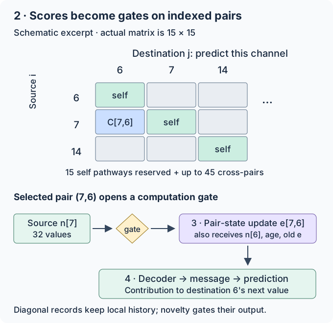
The figure is schematic: shaded cells illustrate a selection, not trained scores. A route record uses (i,j) as its address; its gate controls computation or transmission for that relationship. The token vector is evidence entering the gate, and a learned pairwise prediction is the eventual contribution leaving it.
Keep the diagonal. The complete matrix has \(15\times15=225\) entries. Its fifteen diagonal cells represent self-comparisons. We retain those self pathways explicitly because they provide temporal prediction and novelty signals.
For a concrete budget, reserve one self pathway plus up to three other incoming pairs per destination:
self_records  = 15
cross_records = at_most(15 * 3) = 45
total_records <= 60
There are 210 off-diagonal candidate scores and fifteen diagonal scores; only 45 of those cross-pairs receive expensive pair updates at once. Thus “60 relationships” follows from the budget, not a hidden tensor dimension. In a different experiment, four cross-pairs plus a self record would require 75 slots.
Selection and transmission are separate: the self predictor stays available even when its outgoing novelty gate is closed. Cross-pair gates may start with Top-3 selection per column, then be compared against soft or hybrid selection.
3. Selected pairs update a recurrent relationship record
Take one selected pair, (i,j). It gets a record with a stable pair key, its last-update time, and a 16-value recurrent summary \(e_{ij}\). Think of a small row in a table addressed by (i,j), rather than trying to picture memory living inside a drawn arrow.
| Record field | Concrete content | Purpose |
|---|---|---|
| Pair key | Two indices, e.g. (7,6) |
Identify the source and prediction destination |
Pair state e |
16 learned floating-point values | Summarize this pair’s predictive history |
| Last-update time | Timestamp | Make gaps between updates visible |
| Utility statistics | Running gain/error estimates | Help select, retain, or replace the record |
The raw samples remain in their four-sample buffers. The pair record stores a compressed learned summary, not a growing list of successful sensor samples. Its contents can reflect co-change, lag, or other useful predictive patterns, but those interpretations require measurement.
Using the two current expanded encodings gives a 65-value GRU input: 32 source values, 32 destination values, and one normalized elapsed-time value:
\[\begin{aligned} v_{ij}[t]&=[n_i[t],n_j[t],\tau_{ij}[t]]\in\mathbb R^{65},\\ e_{ij}[t]&=\operatorname{GRU}_{\rm pair}(v_{ij}[t],e_{ij}^{\rm previous}) \in\mathbb R^{16}. \end{aligned}\]pair_input = concat(n[i], n[j], elapsed_since_pair_update / time_scale) # [65]
e[i,j] = pair_gru(input=pair_input, previous_state=e_previous[i,j]) # [16]
For a newly allocated record, initialize the state to zero and mark the current time. Shared GRU weights process every selected pair; each pair keeps its own state. At most sixty records hold 960 pair-state floats. Allocation and expiry policies remain experimental.
Where is the predicted change? The GRU returns e, an intermediate representation. A decoder in stage 4 turns that representation into a proposed change in the destination signal. Prediction error trains both decoder and pair GRU; e itself is not required to equal a change in position or intensity.
We will call increases and decreases in a sensor signal temporal transitions. A graph edge means the indexed relationship (i,j). These two uses of “edge” must not be mixed.
Even a perfectly trained (7,6) record is still organized by sensor indices. It could summarize both a basketball seam and a court line passing those bins. That is a central limitation, returned to in the correspondence section.
4. Decode gated contributions and form destination predictions
The function G is a shared learned feed-forward message decoder. An MLP (multilayer perceptron) here means a learned linear projection, a tanh hidden activation, and a learned linear output. It takes the pair state and source encoding and emits a 16-value predictive contribution:
G = MLP(input_width=48, hidden_width=32, output_width=16)
m[i,j] = G(concat(e[i,j], n[i]))    # 16 pair-state + 32 source values
This message is a learned feature vector derived from the source and its relationship history. A separate output head gives it a directly testable role.
For measured destination \(j\), the self decoder reads local state and its self-pair record. The cross decoder adds a correction:
\[\begin{aligned} \widehat{x}^{\,self}_j[t+1] &=x_j[t]+D_{\rm self}([s_j[t],e_{jj}[t]]),\\ \widehat{x}^{\,ij}_j[t+1] &=\widehat{x}^{\,self}_j[t+1]+D_{\rm cross}([s_j[t],m_{ij}[t]]). \end{aligned}\]self_delta = D_self(concat(s[j], e[j,j])) # 48 -> 1
self_prediction[j] = x[j] + self_delta
pair_correction[i,j] = D_cross(concat(s[j], m[i,j])) # 48 -> 1
pair_prediction[i,j] = self_prediction[j] + pair_correction[i,j]
Both D functions are shared learned MLPs with 48 inputs, a chosen hidden width of 32, and one scalar output. The self pathway forecasts the destination’s change; the cross pathway asks whether additional evidence improves that forecast.
For active cross-pairs, normalize the selected compatibility scores into weights \(\alpha_{ij}\) and combine their scalar corrections:
\[\widehat{x}^{\,combined}_j[t+1] =\widehat{x}^{\,self}_j[t+1] +\sum_{i\ne j:\,gate_{ij}=1}\alpha_{ij}D_{\rm cross}([s_j,m_{ij}]).\]weights = softmax(selected_cross_scores_for_destination_j)
combined_prediction[j] = self_prediction[j] + weighted_sum(pair_corrections)
# If all cross gates are closed, use the self forecast alone.
The original heading called this “messages update the destination.” More precisely, in this sketch messages update the destination’s prediction, while its recurrent local encoder continues to ingest its own observations. This keeps “self history” cleanly separated from cross-channel information. Feeding received messages back into node memory is a separate ablation; if adopted, the self baseline needs a separate local-only state to remain a fair comparator.
We cache each forecast now and judge it only after the next measurement arrives. All messages are computed from information available at the current tick.
5. Evaluate cross-prediction gain and self novelty
Stage 5 closes the learning loop at the next sample. Squared error on normalized raw observations is a simple initial loss:
\[\begin{aligned} \ell^{self}_j[t+1]&=(x_j[t+1]-\widehat{x}^{\,self}_j[t+1])^2,\\ \ell^{ij}_j[t+1]&=(x_j[t+1]-\widehat{x}^{\,ij}_j[t+1])^2,\\ g_{ij}[t+1]&=\ell^{self}_j[t+1]-\ell^{ij}_j[t+1]. \end{aligned}\]actual = next_sample[j]
self_error = squared_error(actual, cached_self_prediction[j])
pair_error = squared_error(actual, cached_pair_prediction[i,j])
gain[i,j] = self_error - pair_error
A positive gain is evidence that this cross-pair added predictive value. It can train future compatibility scores or affect record retention. Forecasts must be cached before the target arrives; selecting pairs using their already-observed next-step error would leak the answer.
The prediction training objective can average self, pair, and combined errors over the measured channels (0–13). Training those losses through the decoders and recurrent states shapes e, s, n, and h. The external action channel is excluded as a prediction target but remains a source of context. The weights between losses, rollout horizon, and routing surrogate require experiments; hard selection itself does not supply gradients to rejected pairs.
The diagonal has another job. Comparing a self forecast with the same forecast gives zero incremental gain, so cross-gain is the wrong survival rule for self pathways. The local self-prediction error is a temporal novelty signal.
One provisional transmission policy smooths that error and emits a self message on novelty onset, sustained novelty at a limited rate, and recovery. Hysteresis uses a higher threshold to turn the gate on than to turn it off:
novelty[j] = smooth(cached_self_error[j])
if quiet[j] and novelty[j] > high_threshold:
    emit_self_event(j, "novelty onset")
    quiet[j] = false
elif not quiet[j] and novelty[j] < low_threshold:
    emit_self_event(j, "novelty subsided")
    quiet[j] = true
elif not quiet[j] and refresh_due(j):
    emit_self_event(j, "still surprising")

# Regardless of transmission, continue the self predictor's local updates.
These are rising/falling novelty transitions, not graph edges. A reliably predicted intensity increase can have little novelty; a static but unexpected signal can have substantial novelty. Noise and undertrained models also produce error, so novelty needs calibration and is not automatically meaningful evidence.
Cross-gain and novelty should both be retained as potential predictive-signature features. Neither is an object-identity certificate or proof of causality. Several individually useful cross-pairs can also be redundant; test combined forecasts and leave-one-pair-out contributions.
The complete toy forward pass
Returning to the overview, here is the dimension ledger for the same five stages. The formerly ambiguous “directional candidates” are simply the entries of the compatibility matrix.
| Stage | Data | Shape or capacity |
|---|---|---|
| 1a | Four-sample scalar buffers | 15 × 4 |
| 1b | Short-pattern features h |
15 × 16 |
| 1c | Expanded encodings n |
15 × 32 |
| 1d | Local recurrent states s |
15 × 32 |
| 2 | Compatibility matrix, diagonal included | 15 × 15 = 225 scores |
| 2 | Self-pair records + selected cross-pair records | 15 + at most 45 = at most 60 |
| 3 | Pair inputs and recurrent states | At most 60 × 65 inputs; 60 × 16 state |
| 4 | Cross messages | At most 45 × 16 |
| 4 | Self / combined forecasts for measured channels | 14 scalars each |
| 4 | Individual cross forecasts for measured destinations | At most 14 × 3 = 42 scalars |
| 5 | Measured errors, gains, and novelty | Per measured destination / evaluated pair |
for each new tick t:
    if cached_forecasts_exist:
        score_forecasts_against_current_measurements()  # stage 5 for t-1

    B = append_samples_to_four_sample_buffers()          # 1a
    h = encode_4_to_16(B)                                # 1b
    n = expand_16_to_32(h)                               # 1c
    s = local_gru(n, previous_s)                         # 1d

    C = compatibility_matrix(s)                         # 2: [15,15]
    pairs = all_self_pairs + up_to_three_cross_pairs_per_destination(C)

    e = update_pair_records(pairs, n, timestamps)        # 3
    forecasts = decode_and_combine(s, e, n, current_x)   # 4
    cache(forecasts, selected_pairs, forecast_timestamp)
    retain(s, e, pair_timestamps, running_statistics)
The capacity is an upper bound. Cross-records targeting the exogenous action channel can be skipped because it is not forecast; then at most 42 cross-records plus fifteen self records are maintained. Keeping the uniform 60-slot allocation makes the bookkeeping simple.
Fifteen local states and sixty pair states require 1,440 FP32 values: 5,760 bytes. Four-sample buffers add 240 bytes. These figures exclude weights, indices, timestamps, cached forecasts, transient tensors, training activations, optimizer state, and allocator overhead. A fixed state size describes bounded storage per slot, not lossless storage of an unlimited history.
The correspondence problem: a design-session placeholder
Status: open theory / interactive design session pending. The single-layer sketch above can learn sensor-level predictive relationships. It does not yet specify how evidence becomes associated with a persistent object.
Return to the basketball and court line. Successfully predicting a change at sensor j from sensor i tells us that a relationship was useful on that transition. Appending or compressing source evidence into j’s state does not say whether it belonged to a basketball, a line, a shadow, or an unrelated object now occupying the same location.
That raises an architectural choice: should persistent evidence be organized by sensor index, by predictive factor, or by a separately maintained entity hypothesis whose participating sensors can change? The first is easy to implement. The other two may be essential to correspondence, but their assignment rules are unresolved. Free association needs structure: allowing arbitrary evidence to mix would simply move the contamination problem.
Theory sketch: sorting unknown parts into provisional piles
Imagine a team sorting parts from five disassembled machines: a robot, a washing machine, a television, a car subsystem, and plumbing. Nobody is given the finished designs.
A person picks up a part, turns it, feels its surfaces, and tries a possible fit. Each small interaction supplies another constraint. The part may join an existing provisional pile, start a new pile, or remain ambiguously associated with several piles. Later evidence can force a split or reassignment.
The useful analogy is incremental evidence assignment under uncertainty. A pile is an evolving hypothesis, not a known object label. Motion, touch, visual structure, and predictive factors may constrain which evidence belongs together. Co-motion alone is insufficient: two separate objects may move together, while one articulated object has parts that move differently.
flowchart TD
    A[/"New sensory evidence and action context"/] --> B{"Which hypothesis fits?"}
    B --> C[("Existing provisional pile")]
    B --> D[("New provisional pile")]
    B --> E["Retain multiple assignments"]
    C --> F["Seek discriminating evidence"]
    D --> F
    E --> F
    F --> A
    F -. contradictions .-> G["Revise, split, or merge"]
    G --> B
This is a question map for the design session, not an implemented sorting algorithm. We still need to specify the message contents, compatibility tests, pile representation, uncertainty, birth/split/merge rules, and how hypotheses communicate across sensory regions.
The Thousand Brains Theory account from Numenta is relevant inspiration: it proposes sensorimotor object models with location context and communication among columns to reach agreement. This is a proposed theoretical framework, not proof that the sketch here solves correspondence. The pertinent lesson for RPR is that agreement about an entity requires a mechanism beyond independent next-signal prediction.
Desired efficiency: a bounded amount of work per arriving observation, even after much evidence has accumulated. Fixed-size recurrent summaries can bound memory per hypothesis, but they compress information and can forget. Constant work also requires bounded candidate retrieval and a policy for hypothesis capacity; comparing every new observation with every accumulated pile grows with the number of piles. The trade-off between bounded compute, ambiguity, and revisiting old evidence is part of the open problem.
The next design session should follow one part—or one moving patch—through several observations and answer: Which record receives this evidence, why that record, and what evidence would make us reverse the assignment?
Recursion is a later question
First establish one layer’s evidence semantics, learning objective, and correspondence mechanism. Adding layers before those are clear risks hiding the same ambiguity inside larger latent vectors.
A future layer could receive summaries of predictive factors or provisional entity hypotheses. It would execute the same kind of operations with its own inputs and persistent state. That does not imply copying activations or sharing network weights. Promotion rules, timescales, and downward control interfaces remain future design work.
PCFH provides a vocabulary for learned factors and composition. Whether those factors supply the right grouping unit is a concrete question to revisit after the single-layer experiment.
What RPR currently specifies
The working sketch specifies local temporal encoding, a compatibility matrix, gates on indexed pairs, recurrent pair summaries, and prediction-based training signals. It proposes distinct policies for cross-prediction gain and self novelty.
The broader ambition is coherent evidence accumulation. That remains an architectural requirement rather than a demonstrated consequence of these components.
What is incomplete
The following ten criteria are intended to remain fixed across iterations. These are editorial maturity ratings, not measured performance or probabilities that the theory is correct. The scale is: 0 = requirement identified but mechanism missing; 1 = a candidate mechanism is described; 2 = implemented with reproducible checks; 3 = supported by controlled baseline comparisons. A changed definition must be versioned rather than silently moving the goalposts.
| ID | Fixed criterion | Revision 2 rating | Evidence for rating / what would advance it |
|---|---|---|---|
| C1 | Dataflow and state semantics | 1 | Explicit B → h → n → s → C → e → prediction; needs executable shape/time checks |
| C2 | Single-layer predictive learning | 1 | Raw-target loss and decoder roles defined; needs trained held-out predictions |
| C3 | Routing credit and useful sparsity | 1 | Compatibility gates and delayed gain proposed; needs workable exploration and matched-compute tests |
| C4 | Self novelty and uncertainty | 1 | Self pathway retained; hysteresis candidate; needs noise-calibration tests |
| C5 | Temporal correspondence and identity | 0 | Sensor-pair states do not specify identity assignment; needs an explicit assignment mechanism |
| C6 | Multi-sensor agreement and evidence grouping | 0 | Provisional-pile analogy only; needs a representation and message/consensus protocol |
| C7 | State lifecycle and contamination control | 0 | Birth/expiry/reset/split semantics unresolved; needs lifecycle rules and boundary tests |
| C8 | Bounded inference memory and latency | 1 | Single-layer capacity budget stated; needs actual latency/memory measurements and bounded hypothesis retrieval |
| C9 | Action-conditioned prediction and causal control | 1 | Applied command is an input; causal attribution and stable control still need interventions and a controller |
| C10 | Falsifiability and comparative evaluation | 1 | Tests and baselines specified below; needs runnable experiments and reported outcomes |
Evaluation log: 2026-09-22, Revision 2, criterion version 1. This is the first recorded assessment; do not invent numeric ratings for the earlier article. In subsequent revisions keep these IDs, append dates and evidence, and explain score changes. There is intentionally no combined score: improvements in predictive loss cannot compensate for missing identity semantics.
Route learning and credit assignment
Hard Top-K selects a bounded number of pairs but does not differentiate through the selected indices. Selected pairs receive training while rejected pairs may never get a chance to improve. A router could learn from cached gain on explored pairs, but needs exploration and a clearly specified delayed credit rule.
Soft routing permits uncertain mixtures and gradient-based weight updates, yet dense scoring and updates can be expensive. Sparse candidate retrieval followed by soft gates, or a bounded set of competing assignments, are useful alternatives to test. The messy ambiguity in the sorting analogy is a genuine requirement, not merely an inconvenience to remove with a winner-takes-all operation.
Edge lifecycle
A graph-edge record currently stores the (i,j) key, learned pair summary, elapsed time, and utility statistics described in stage 3. The working forward pass keeps it by sensor-pair address; it has no object-ownership field or successful-evidence log.
We have not chosen how to preserve, expire, reset, or reassign a record when a pair becomes inactive or when a new scene uses the same sensors. Holding state indefinitely risks mixing entities; immediate reset loses useful continuity. An entity- or factor-indexed evidence store would need its own assignment mechanism before this lifecycle could be defined coherently.
Fair self-versus-cross comparison
Keep the self state local-only, give both models the same prediction horizon, and compare on held-out sequences. Match or report parameter budgets and inference work. A larger cross decoder can outperform a smaller self decoder for reasons unrelated to the source evidence. Test shuffled-source and unrelated-source controls, and whether individual gains survive joint aggregation.
Higher-level node creation
Deferred until one layer has a tested interpretation. Compression alone does not define which factors belong together or which variables a higher-level interface must preserve.
Control and causality
An action stream can help predict a consequence without identifying the true controllable mechanism. Randomized interventions, delays, hidden disturbances, and system changes are required tests. A controller, safety constraints, and a control objective are additional components; the scripted camera path supplies none of them.
Tracking under occlusion and ambiguity
No current mechanism binds an interrupted stream back to a continuing entity. Identical objects, crossing trajectories, and occlusions should remain explicit failure cases until a correspondence design exists.
Open questions
- Should
nremain a separate expansion, or can one recurrent encoder replace both projections without losing useful structure? - What does pair state retain that a matched-capacity local recurrent model cannot?
- Which record should accumulate evidence when the sensor index stays fixed but the observed entity changes?
- What evidence justifies starting, splitting, merging, or revisiting a provisional pile?
- How should visual, tactile, and proprioceptive hypotheses communicate about a common entity?
- Can cross-gain and self-novelty be calibrated without starving quiet but important relationships?
- How can candidate retrieval remain bounded as object hypotheses accumulate?
- Which predictive factors would constrain evidence grouping without incorrectly equating correlation with common identity?
Principal risks
- Identity mixing: ball and court-line evidence remain blended despite low prediction error.
- Graph churn and starvation: selections change too quickly, or early lucky pairs monopolize updates.
- Redundant evidence: several high-gain pairs repeat the same clue rather than provide independent support.
- False novelty: noise, camera motion, or an undertrained model dominate self-event traffic.
- Stale state: old pair summaries contaminate new scenes.
- Compression loss: finite recurrent state forgets distinctions needed for later reassignment.
- Hidden compute growth: dense pair scoring or an expanding pile search overwhelms the sparse update budget.
- Causal confusion: a useful predictor is mistaken for a reliable control pathway.
- Premature hierarchy: more layers obscure single-layer defects.
- Evaluation leakage: giving the learner “target” channels or evaluating on the scripted path falsely suggests correspondence has been learned.
The first falsifiable experiment
First build a prediction-only benchmark with randomized camera trajectories and scene configurations, using the unlabeled sensor inputs above. Split by entire scenes/trajectories, not adjacent frames. Train on more than the six illustrated states.
Compare:
- A last-value predictor and a feed-forward model over the four-sample windows.
- A flat GRU with access to the same information.
- Independent per-sensor recurrent predictors.
- The single-layer RPR sketch with self and cross records.
- Ablations removing pair recurrence, cross-gain supervision, or novelty gating.
- Hard gates versus soft gates under matched or explicitly reported compute budgets.
Measure raw next-step and rollout error, cross-source utility, route churn, novelty false-positive rate, latency, memory, and sensitivity to camera gain/delay changes. Test against stronger baselines, not only a weak self predictor.
Separately test correspondence. Build the basketball-seam → court-line counterexample; use two identical moving objects; hide and reintroduce an object; and later add visual/tactile observations of the same versus different things. Ground-truth identities belong only to evaluation, not to the input channels. Once a model exposes assignment hypotheses, measure identity switches, false merges/splits, recovery after occlusion, and contradictory evidence accumulation alongside prediction loss. Until then, record correspondence as not implemented, rather than treating good pixel forecasts as a passing result.
The decisive outcome could be low prediction error with poor or undefined identity consistency. That would show exactly where predictive routing stops short of the intended architecture.
Current conclusion: RPR has a more explicit single-layer predictive computation to investigate. Coherent evidence assignment—the mechanism that turns streaming observations into provisional, revisable “piles”—is the next design problem, not a benefit already obtained from recurrence.
References and implementation boundaries
- Cho et al., 2014: Learning Phrase Representations using RNN Encoder–Decoder introduces the gated recurrent unit used here as one candidate temporal encoder. This supplies a standard building block, not evidence for RPR.
- Numenta: The Thousand Brains Theory of Intelligence explains its proposed location-based sensorimotor models and voting between models. It motivates the correspondence discussion without settling RPR’s design.
- PCFH: variables to predictive factors is the related factor/composition proposal on this site.