<?xml version="1.0" encoding="utf-8"?><feed xmlns="http://www.w3.org/2005/Atom" ><generator uri="https://jekyllrb.com/" version="3.10.0">Jekyll</generator><link href="https://spencerbug.github.io/feed.xml" rel="self" type="application/atom+xml" /><link href="https://spencerbug.github.io/" rel="alternate" type="text/html" /><updated>2026-10-08T18:14:10+00:00</updated><id>https://spencerbug.github.io/feed.xml</id><title type="html">Spencer Neilan</title><subtitle>Embedded Linux, platform firmware, low-level systems, networking, embedded security, and embodied intelligence.</subtitle><entry><title type="html">MORPH, Part 2: Good Predictions, Inconsistent Coordinates</title><link href="https://spencerbug.github.io/blog/morph-part-2/" rel="alternate" type="text/html" title="MORPH, Part 2: Good Predictions, Inconsistent Coordinates" /><published>2026-10-08T17:00:00+00:00</published><updated>2026-10-08T17:00:00+00:00</updated><id>https://spencerbug.github.io/blog/morph-part-2</id><content type="html" xml:base="https://spencerbug.github.io/blog/morph-part-2/"><![CDATA[<aside class="author-note" role="note">
  <strong>Author’s note:</strong> I use AI as a writing and research tool while developing these ideas. The architecture, hypotheses, questions, and technical review are my own. This is exploratory work, not a peer-reviewed result.
</aside>

<p><strong>Research update · completed experiment plus untested directions.</strong> This follows <a href="/blog/morph/">MORPH: Model of Object Representation and Predictive Homomorphisms</a>. The measurements below come from the completed O1 campaign. The populations, moving sensors, and recurrent hierarchy discussed afterward have not been implemented or evaluated in that campaign.</p>

<p>MORPH started with an ambitious question: can an agent build persistent object models whose representations change predictably when it acts? The first experiments reduced that question to something much smaller: encode a simple image, rotate part of its embedding, and decode the expected rotated view.</p>

<p>The latest result is encouraging and incomplete. We now have a model that reconstructs geometric shapes and predicts their rotated views accurately on new instances of familiar shape families. But the encoder does not produce sufficiently consistent pose coordinates across those views. All five final seeds passed 18 of 19 registered checks. The same remaining check failed in every seed.</p>

<p>That is a negative result for the full experiment. It is also a useful separation of two things I had initially hoped would improve together: good image prediction and a dependable internal coordinate system.</p>

<h2 id="what-o1-actually-tested">What O1 actually tested</h2>

<p>O1 was a bounded architecture and optimization search, not the complete MORPH system. It used synthetic white geometric silhouettes on black backgrounds, rendered with antialiasing to 32 × 32 pixels. The familiar families included ellipses, polygons, concave shapes, holed shapes, and unions of primitives.</p>

<p>The learner received an initial image and known rotation increments in radians. It predicted future views without receiving the intervening target images as inputs. Training included reconstruction and prediction at horizons 1, 2, 4, and 8, plus feature-invariance and pose-equivariance losses. There was no object memory, ownership inference, recurrence, or learned motor calibration.</p>

<p>The encoder split its output into two parts:</p>

<ul>
  <li>An <strong>invariant feature code</strong>, intended to retain information that survives rotation.</li>
  <li>An <strong>equivariant pose code</strong>, intended to change in a prescribed way under rotation.</li>
</ul>

<p>Those names describe training objectives. They do not prove that one branch contains pure identity and the other contains pure pose.</p>

<p>The selected recipe used a fully connected encoder with separate feature and pose heads, followed by a convolutional decoder. Its latent contained 32 invariant values and 32 pose values. The pose values formed 16 disjoint coordinate pairs, with four pairs assigned to each harmonic from 1 through 4.</p>

<p>Each pair rotates by its harmonic times the supplied angle. These are rotations of activation coordinates in the embedding, not rotations of the network’s learned weights. The group action is fixed; the encoder and decoder must learn to work with it.</p>

<p>The search evaluated 24 configurations across three encoder families: convolutional encoders with separate dense heads, convolutional encoders with a shared projection and output split, and fully connected encoders with separate heads. Two finalists were evaluated across five seeds, with one recipe selected using validation data before the final audit. This does not establish that dense encoders are generally better than convolutional encoders.</p>

<p>The complete campaign consumed 260,000 optimizer updates and 20.83 accounted hours, within its authorized 55-hour cap. Source, data, and checkpoint hashes were frozen, and 4,960 saved prediction tickets were checked for prediction-before-score chronology. That establishes an auditable run; it does not turn an unsuccessful criterion into a successful one.</p>

<h2 id="the-measured-result">The measured result</h2>

<p>The primary frozen test contained 512 new objects drawn from familiar shape families.</p>

<table>
  <thead>
    <tr>
      <th>Measurement</th>
      <th style="text-align: right">Final result</th>
    </tr>
  </thead>
  <tbody>
    <tr>
      <td>Reconstruction foreground MSE, range across five seeds</td>
      <td style="text-align: right">0.00463–0.00582</td>
    </tr>
    <tr>
      <td>Eight-step foreground MSE, mean across seeds</td>
      <td style="text-align: right">0.00717</td>
    </tr>
    <tr>
      <td>Eight-step MSE, 95% bootstrap interval</td>
      <td style="text-align: right">0.00657–0.00780</td>
    </tr>
    <tr>
      <td>Normalized pose-consistency ratio, range across seeds</td>
      <td style="text-align: right">0.272–0.334</td>
    </tr>
    <tr>
      <td>Required pose-consistency ratio</td>
      <td style="text-align: right">≤ 0.10</td>
    </tr>
    <tr>
      <td>Registered checks passed</td>
      <td style="text-align: right">18 of 19 in every seed</td>
    </tr>
  </tbody>
</table>

<p>MSE is mean squared pixel error on intensities from zero to one. The foreground metric uses a renderer-defined support mask; prediction comparisons use the union of source and target foreground. These masks are evaluator information, not learner inputs. Scores are aggregated with family and action-schedule balancing. The confidence interval uses paired seed/family-object bootstrap resampling. An MSE of 0.11 is not an 11% classification error.</p>

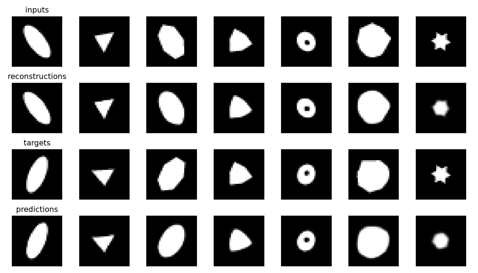
<p><img src="/assets/morph-part-2/o1-examples.png" alt="O1 model outputs: source images, reconstructions, rotated targets, and predicted rotated views. The final column shows a difficult shape losing its tips." /></p>

<p><em>Saved model outputs from the final report, not a scripted illustration. The panel shows seed 0 on the primary test: the first object from each family and the worst object by eight-step foreground error. Rows show inputs, reconstructions, eight-step targets, and predictions. The final column makes a failure visible: the model rounds away the shape’s protrusions.</em></p>

<p>The distinction between kinds of unseen data matters. New instances from familiar families performed well. Entirely withheld families performed substantially worse:</p>

<table>
  <thead>
    <tr>
      <th>Separate diagnostic distribution</th>
      <th style="text-align: right">Eight-step foreground MSE, range across seeds</th>
    </tr>
  </thead>
  <tbody>
    <tr>
      <td>Withheld families: crescents and curved strips</td>
      <td style="text-align: right">0.083–0.110</td>
    </tr>
    <tr>
      <td>Historical grayscale three-ellipse objects</td>
      <td style="text-align: right">0.068–0.099</td>
    </tr>
    <tr>
      <td>Controlled symmetry set</td>
      <td style="text-align: right">0.058–0.073</td>
    </tr>
  </tbody>
</table>

<p>These diagnostic distributions were excluded from recipe selection and primary acceptance. Their errors limit the claim: O1 learned useful prediction within a distribution, not broad geometric generalization.</p>

<h2 id="how-can-the-pixels-be-right-while-the-coordinates-are-wrong">How can the pixels be right while the coordinates are wrong?</h2>

<p>Let E be the encoder, D the decoder, u the feature code, and p the pose code. Let R rotate the actual image by angle theta, and let rho apply the prescribed rotation to the pose code. The desired relationship is:</p>

\[p(R_\theta x) \approx \rho(\theta)p(x).\]

<p>In words: rotating the image and then encoding it should produce approximately the same pose code as encoding it first and rotating that code. The reported pose ratio normalizes the root-mean-square discrepancy by within-object pose-code variation across views, on objects whose rendered views change. It is not an angular error or a percentage of incorrect poses.</p>

<p>The decoded prediction instead tests:</p>

\[D\bigl(u(x),\rho(\theta)p(x)\bigr) \approx R_\theta x.\]

<p>These are different requirements. A decoder can map several different latent codes to similar images. Consequently, good reconstruction and good prediction do not guarantee that the two latent routes agree. Our aggregate image scores also do not prove that the routes decode identically on every example.</p>

<p>Two explanations remain open. The discrepancy might lie mostly in redundant directions that barely affect decoded pixels. Alternatively, the decoder might compensate for a meaningful mismatch between the encoder and the prescribed transformation. Both could occur together. We have not yet measured which dominates.</p>

<p>Replacing either the feature or pose branch damaged predictions, so both branches are being used. But replacement can create codes outside the training distribution. It is not proof of clean disentanglement.</p>

<p>There is another distinction here: our rotation matrices already satisfy the group composition law by construction. Applying two rotations composes correctly. What failed was the learned encoder’s alignment with those rotations. A later memory or planning module consuming the latent directly may care about that discrepancy even if the image decoder can tolerate it.</p>

<h2 id="what-the-homomorphism-autoencoder-paper-establishes">What the homomorphism autoencoder paper establishes</h2>

<p><a href="https://proceedings.mlr.press/v202/keurti23a/keurti23a.pdf">Keurti et al.’s Homomorphism Autoencoder</a> learns action representations jointly with observation representations. Its toroidal translation experiment uses discrete cyclic x/y shifts, corresponding to a subgroup of SO(2) × SO(2). It reports separate rotation blocks for those axes, a further rotation factor in another setting, identity separation among three shapes, and 128-step prediction after training on two-step trajectories. It also studies SO(3) rotations of a 3D bunny.</p>

<p>Those are stronger demonstrations of learned transformation structure than O1 currently provides. But the paper does not report our normalized pose-consistency gate, and its BCE reconstruction measurements cannot be numerically ranked against our foreground MSE. A matched reproduction is needed to compare performance directly.</p>

<p>The torus also clarifies a possible next task. Horizontal and vertical wraparound movement are two independent circular coordinates. Our current harmonics all respond to one rotation angle; adding more harmonics does not create an independent movement axis.</p>

<h2 id="could-populations-tolerate-imperfect-consistency">Could populations tolerate imperfect consistency?</h2>

<p>One possibility is to represent several plausible poses instead of forcing one estimate. This becomes especially relevant for a tiny moving sensor: a patch showing a straight edge may correspond to several places on an object.</p>

<p>A population could retain candidate locations and weights. Movement transports those candidates; each predicts a future patch; new pixels change their weights. Agreement between sensors would mean that their hypotheses support compatible object states after accounting for relative sensor positions. Equal confidence scores alone would not mean agreement.</p>

<p>This is an untested hypothesis for MORPH. It might help if a single-state model fails because observations are genuinely ambiguous. It would not automatically remove redundant latent coordinates or repair a systematically wrong action model. We have not established ambiguity as the cause of O1’s failed gate.</p>

<p>A single Gaussian describes uncertainty around one region. Multiple distinct explanations may require multiple peaks or an explicit weighted population, especially when pose wraps around. The useful outcome would be accurate predictions and appropriate uncertainty reduction as new evidence arrives. A distribution that simply widens enough to accommodate everything would not be a success.</p>

<p>O1’s failed gate should remain failed. A population experiment would need its own registered question and criteria, including whether the correct alternative survives an ambiguous sequence and gains support when a distinguishing landmark appears.</p>

<h2 id="from-moving-patches-to-a-shared-recurrent-model">From moving patches to a shared recurrent model</h2>

<p>Another direction is to move a small sensor over a hidden image and accumulate its glimpses. Imagine seeing a duck through a pinhole. A recurrent encoder could retain observations and displacement information, while a decoder reconstructs the larger region.</p>

<p>Two capabilities must be measured separately. Remembering and placing pixels already observed is spatial memory; a canvas that pastes patches at known coordinates is an essential baseline. Predicting the unseen body from a glimpse of the beak is learned completion and should remain uncertain. A plausible invented duck is not the same as recovering the hidden image.</p>

<p>Multiple local recurrent encoders could then feed a parent recurrent autoencoder. The parent would receive child embeddings and their relative positions, compress them into a larger-scale state, and reconstruct or predict the child observations. Joint training would let parent prediction errors encourage child representations that are easier to combine, while local reconstruction would protect detail.</p>

<p>The following is a proposed computation, not an implemented model:</p>

<pre><code class="language-mermaid">flowchart TD
    O["1. New patches and displacement"] --&gt; C["2. Local recurrent encoders"]
    L["Previous local memories"] --&gt; C
    C --&gt; P["3. Parent recurrent encoder with relative positions"]
    H["Previous parent memory"] --&gt; P
    P --&gt; D["4. Predict future child patches"]
    D --&gt; S["5. Freeze predictions, then score newly revealed pixels"]
    C --&gt; L
    P --&gt; H
</code></pre>

<p>Reconstructing embeddings that the parent just received tests compression. Predicting withheld or future patches tests whether it learned useful relationships. Pixel-level checks remain necessary: an embedding-only objective could improve because the children discard information.</p>

<p>Shared weights alone do not establish a shared object model or coordinate frame. Two paths ending at the same location should support compatible predictions, but their memories can legitimately differ if one path gathered more evidence. The parent’s identity hypothesis can help interpret local patches; its persistence is not independent confirmation that the identity is correct.</p>

<p>Likewise, a parent prediction sent back to a child is context, not a new observation. Recurrent feedback must not count the same evidence repeatedly. That discipline from the original MORPH proposal becomes more important as the hierarchy grows.</p>

<h2 id="what-should-earn-the-next-layer">What should earn the next layer?</h2>

<p>Stacking this pattern across spatial and temporal scales is an appealing direction. Each level could retain features, track transformations, accumulate uncertain evidence, and predict the level below. But longer timescales need explicit objectives, and actions involving contact, deformation, or irreversible change will need dynamics beyond group rotations.</p>

<p>The immediate research choices are smaller. A frozen-model diagnostic can determine whether O1’s actual latent discrepancies affect decoded geometry. A moving-patch experiment can test whether recurrence retains observed detail and improves future prediction. A population comparison can isolate the value of preserving ambiguity. A two-level comparison can test whether parent feedback helps beyond a flat recurrent model with comparable information and capacity.</p>

<p>These should be separate, registered tests rather than one large system whose failures are impossible to attribute. None has started as part of this update.</p>

<p>The useful advance is concrete: structured prediction now works reasonably well for familiar geometric families. The unresolved issue is equally concrete: accurate output has not yet given us the common internal coordinates MORPH would like to use. The next mechanisms need to earn their place by explaining or overcoming that limitation, with new observations providing the evidence.</p>]]></content><author><name></name></author><summary type="html"><![CDATA[The first bounded MORPH optimization campaign predicts rotated shapes well but misses latent equivariance. What worked, what failed, and why recurrent populations and patch hierarchies remain hypotheses.]]></summary></entry><entry><title type="html">MORPH: Model of Object Representation and Predictive Homomorphisms</title><link href="https://spencerbug.github.io/blog/morph/" rel="alternate" type="text/html" title="MORPH: Model of Object Representation and Predictive Homomorphisms" /><published>2026-09-28T14:46:00+00:00</published><updated>2026-10-08T00:00:00+00:00</updated><id>https://spencerbug.github.io/blog/temporal-escrow-resonance</id><content type="html" xml:base="https://spencerbug.github.io/blog/morph/"><![CDATA[<aside class="author-note" role="note">
  <strong>Author’s note:</strong> I use AI as a writing and research tool while developing these ideas. The architecture, hypotheses, questions, and technical review are my own. This is exploratory work, not a peer-reviewed result.
</aside>

<p><strong>Experimental follow-up:</strong> <a href="/blog/morph-part-2/">MORPH, Part 2: Good Predictions, Inconsistent Coordinates</a> reports the completed O1 campaign and separates its measured findings from proposed recurrent and population-based extensions.</p>

<p><strong>Working research note · architecture under active review.</strong> MORPH — Model of Object Representation and Predictive Homomorphisms — is an exploratory architecture, not an experimentally validated model. It grew out of a narrower question about object identity: how can an embodied learner continuously create new identities, learn from them aggressively, and still prevent its own recurrent hypotheses from returning as counterfeit evidence?</p>

<p>The proposal has now sharpened into three coupled problems:</p>

<ol>
  <li><strong>Persistent identity:</strong> create a new object memory immediately, without adding a new classifier output or retraining the whole network.</li>
  <li><strong>Structured sensorimotor dynamics:</strong> use one shared equivariant encoder so actions move a representation along lawful, compositional transformation trajectories rather than through an arbitrary next-state predictor.</li>
  <li><strong>Controlled plasticity:</strong> when gradient descent improves the encoder, migrate old memories and learned dynamics into the new representational coordinates instead of silently invalidating them.</li>
</ol>

<p>The central proposal is:</p>

<blockquote>
  <p><strong>Persistent identities should be fast nonparametric memories interpreted by a shared equivariant predictive substrate. Physical action should induce structured motion through that substrate. When the substrate itself changes, old knowledge should migrate through an explicit compatibility transform and the update should remain in escrow until both old identities and old dynamics still work. A hypothesis may influence what is predicted or tested next, but evidence used to create that hypothesis cannot also validate it.</strong></p>
</blockquote>

<p>This separates three jobs:</p>

<ol>
  <li><strong>Fast memory</strong> creates and updates individual object hypotheses without gradient descent.</li>
  <li><strong>Fast equivariant dynamics</strong> map actions into predictable transformations of patch representations.</li>
  <li><strong>Slow shared plasticity</strong> updates the encoder, decoder, identity–pose factorizer, group-action model, retrieval metric, vigilance machinery, grouping machinery, and later abstraction layers under anti-forgetting constraints.</li>
</ol>

<p>The decoder is part of the predictive substrate: it maps a predicted future embedding back into real sensor space so the prediction can be compared with what the robot actually sees or feels. MORPH’s relationship to Homomorphism AutoEncoders is discussed in <a href="#comparison-with-homomorphism-autoencoders">section 15</a>.</p>

<p>MORPH therefore tries to preserve several attractive properties at once:</p>

<ul>
  <li>one-shot or few-shot creation of a previously unknown identity;</li>
  <li>broad gradient updates that improve general machinery across many identities;</li>
  <li>action-conditioned prediction that reuses geometric structure instead of relearning every transition independently;</li>
  <li>explicit migration of old memories when the learned representation changes;</li>
  <li>temporal evidence accounting that prevents recurrent hypotheses from validating themselves.</li>
</ul>

<p>Two different transformation structures appear and should not be conflated.</p>

<p>The <strong>physical transformation group</strong> describes lawful action and motion, for example \(SE(3)\) for rigid 3-D rotation and translation. Its action on the learned representation predicts how features should move when the camera, robot, or object moves.</p>

<p>The <strong>representation-migration group</strong> describes a change of coordinates between encoder versions. A useful first approximation is an orthogonal transform in feature space. It need not be the same group as the physical motion model.</p>

<p>The first toy architecture still begins with fixed sensor patches, sparse approximate-nearest-neighbor retrieval, ART-like vigilance, active experiments, and an unknown number of persistent identities. The longer-term hypothesis is that the same proposal/challenge/resonance and controlled-migration rules can recurse into parts, objects, relations, scenes, affordances, and still higher abstractions.</p>

<h2 id="1-the-problem-open-ended-identity-without-local-only-learning">1. The problem: open-ended identity without local-only learning</h2>

<p>A conventional classifier usually ends in a fixed output vector:</p>

\[p(y\mid x)
=
[p(C_1),p(C_2),\ldots,p(C_K)].\]

<p>That assumes the identity vocabulary is known when the model is built.</p>

<p>An embodied learner has a different problem. It may encounter object \(K+1\) tomorrow, \(K+2\) next week, and millions more over its lifetime. Rebuilding and retraining a softmax head whenever a new identity appears is the wrong abstraction.</p>

<p>A more natural starting point is a shared encoder:</p>

\[z = E_\theta(x),\]

<p>with persistent identities represented separately in memory:</p>

\[M_1,M_2,\ldots,M_K.\]

<p>A new object can then be created by allocating a new memory artifact rather than a new output neuron.</p>

<p>But this creates a second problem.</p>

<p>If every persistent identity owns its own private predictor, matcher, or transition model, then experience with one object updates only that object. Learning becomes narrow. A new observation does not improve the machinery used by thousands of related and unrelated things.</p>

<p>That loses one of the major strengths of deep learning:</p>

<blockquote>
  <p><strong>A single prediction error can update a large shared parameter set simultaneously.</strong></p>
</blockquote>

<p>MORPH therefore deliberately makes persistent identities mostly <strong>memory</strong>, while keeping most trainable machinery <strong>shared</strong>.</p>

<h2 id="2-architecture-at-a-glance">2. Architecture at a glance</h2>

<p>MORPH uses a shared representation with an explicit <strong>identity–pose factorization</strong>. Here, identity means a persistent individual thing; pose latent means the current view or transformation state relative to learned anchors. It need not be a calibrated position and orientation in meters and radians.</p>

<pre><code class="language-mermaid">flowchart TD
    X["1. Sensor patch histories"] --&gt; E["2. Shared equivariant encoder"]
    E --&gt; Z["3. Joint latent field"]
    Z --&gt; F["4. Joint grouping and identity–pose inference"]
    F --&gt; I["Identity descriptor and candidate memory"]
    F --&gt; P["Pose latent and ownership uncertainty"]
    I --&gt; ANN["5. ANN candidates plus UNKNOWN"]
    ANN --&gt; H["6. Competing instance hypotheses"]
    P --&gt; H
    H --&gt; D["7. Transform latent and decode predicted observation"]
    D --&gt; T["8. Freeze prediction, act, then score new evidence"]
    T --&gt; M["9. Update memory without gradients"]
    M --&gt; ANN
    T --&gt; U["10. Train candidate shared model"]
    U --&gt; R["Review old identities, dynamics, and migration"]
    R --&gt; E
</code></pre>

<p>Stages 1–3 encode the observation before assigning object ownership. Stages 4–6 keep competing identity, grouping, and pose explanations. Stages 7–9 test those explanations against future observations. Stage 10 improves the shared machinery only after scoring, with a separate review before deployment.</p>

<p>For patch \(i\) at time \(t\), the encoder produces:</p>

\[z_{i,t}=E_\theta(x_{i,t-L:t}).\]

<p>The input is a history of length \(L+1\). Its population code over patches is:</p>

\[Z_t=\{z_{i,t}\}_i.\]

<p>A factorizer \(F_\eta\), using that field and provisional ownership weights \(w_{ij,t}\), proposes:</p>

\[(u_{j,t},p_{j,t})=F_\eta(Z_t,w_{j,t}).\]

<p>Here \(u_j\) is an approximately invariant identity descriptor and \(p_j\) is the pose latent for candidate instance \(j\). Ownership and factorization are refined together; neither is assumed known initially. A local retrieval head can still produce coarse patch keys \(k_{i,t}=I_\phi(z_{i,t})\), but those are candidate cues rather than complete invariant object identities.</p>

<p>A composition function \(C_\eta\) combines identity and pose into an object latent. For group-modeled motion:</p>

\[\hat p_{j,t+1}=\rho_p(g_{j,t})p_{j,t},
\qquad
\hat z^{\mathrm{group}}_{j,t+1}
=C_\eta(u_{j,t},\hat p_{j,t+1}).\]

<p>The group element is \(g_{j,t}=\exp(\xi_{j,t}\Delta t)\), with generator \(\xi_{j,t}=f_\psi(a_t,c_t,H_{j,t})\). Context \(c_t\) includes available motion and sensor information; the hypothesis \(H_{j,t}\) specifies candidate ownership and relative state. A motor command does not directly specify every object’s motion.</p>

<p>The composition is constrained to respect the group:</p>

\[C_\eta(u,\rho_p(g)p)\approx\rho_z(g)C_\eta(u,p).\]

<p>An additional shared dynamics residual \(r_\omega\) predicts effects outside that model:</p>

\[\hat z_{j,t+1}
=\hat z^{\mathrm{group}}_{j,t+1}
+r_\omega(z_{j,t},a_t,c_t,H_{j,t}).\]

<p>A shared decoder \(D_\delta\) maps the predicted latent field \(\hat Z_{t+1}\), predicted ownership/visibility \(\hat W_{t+1}\), and sensor context back to real observation space:</p>

\[\hat x_{t+1}
=D_\delta(\hat Z_{t+1},\hat W_{t+1},c_t).\]

<p>For vision, this means image intensities or a distribution over pixels; touch and other sensors need corresponding outputs. This is the sensor-space prediction, not another identity key. A spatial decoder must handle features moving between patches and visibility changes; the same fixed patch does not necessarily observe the same surface at the next time step. An object-centered decoder alone needs a projection/compositing step to predict the camera image.</p>

<p>Persistent memory stores identity descriptors, view/orbit anchors, transition traces, encoder versions, relations, and uncertainty. It supplies data interpreted by shared functions, rather than a private deep network for each object.</p>

<p>Encoder evolution has a separate compatibility transform:</p>

\[E_{\theta'}(x)\approx Q E_\theta(x)+u_{\mathrm{new}}(x).\]

<p>The transform \(Q\) carries old coordinates forward; \(u_{\mathrm{new}}\) denotes candidate new representational capacity. For a first migration model, \(Q=\exp(A)\) with \(A^\top=-A\). New capacity and the mismatch left after fitting \(Q\) are distinct from the dynamics residual.</p>

<h2 id="3-fixed-sensor-patches-and-sparse-identity-retrieval">3. Fixed sensor patches and sparse identity retrieval</h2>

<p>The first toy version divides the visual field into fixed patches. Each patch encodes a short history into a compact population code \(z_{i,t}\), then proposes sparse local matches:</p>

\[k_{i,t}=I_\phi(z_{i,t}),
\qquad
C_i=\operatorname{ANN}_K(k_{i,t}).\]

<p>For example, patch 17 might retrieve objects 42, 781, 19, and 103, plus <strong>UNKNOWN</strong>. The index searches stored local prototypes and maps each hit back to its parent identity. Different patches can retrieve different sets; a global list of every identity is unnecessary.</p>

<h3 id="from-a-variant-patch-to-an-invariant-identity">From a variant patch to an invariant identity</h3>

<p>An equivariant encoder does not automatically deliver a unique object ID. A small patch showing a uniform blue surface may belong to a stapler, a mug, or a wall. No transformation matrix can recover identity information that the observation does not contain.</p>

<p>The desired relationships are:</p>

\[E(g\cdot x)\approx\rho(g)E(x),
\qquad
I_\phi(\rho(g)z)\approx I_\phi(z).\]

<p>The first retains predictable transformation information. The second reads out information stable under the modeled transformations. A readout can learn that stability from reliably associated views without receiving the absolute pose at inference time. It can also marginalize over candidate transformations or compare multiple stored views. Invariance alone is insufficient: a constant output is invariant too, so reconstruction and discrimination constraints must preserve useful information.</p>

<p>For realistic 3-D objects, rotation changes visibility and can move evidence across patch boundaries. A fixed crop is generally not closed under the object’s rotation group. Consequently, the exact equations apply most cleanly to an object-centered latent or the whole latent field with correspondence, while local patch keys are only approximate, partial evidence.</p>

<p>MORPH therefore proposes a bounded joint inference loop:</p>

<ol>
  <li><strong>Retrieve locally:</strong> appearance, short-term continuity, and stored view anchors generate candidate identities without requiring a known pose.</li>
  <li><strong>Propose ownership:</strong> neighboring patches and coherent motion support several possible instance groupings.</li>
  <li><strong>Infer pose per candidate:</strong> compare the grouped evidence with candidate anchors, retaining alternative poses or axes when ambiguous.</li>
  <li><strong>Predict and challenge:</strong> test each identity–ownership–pose explanation through future views or actions; only afterward update persistent memory.</li>
</ol>

<p>This resolves the execution-order circularity by keeping alternatives, rather than assuming identity must be settled before pose or grouping can be estimated. It does not guarantee a correct or efficient solution. The cost is limited by candidate counts and recurrence budgets, and ambiguous observations may remain unknown.</p>

<p>A rotation is also defined relative to a frame and origin. Rotating about an unknown object center is not necessarily a rotation about the camera origin. A rigid transform must include the corresponding translation, and relative camera/object motion must be inferred or measured. The pose latent can encode those relationships without initially exposing metric coordinates. One shared motion hypothesis must coordinate the population code; arbitrary independent rotations of each feature vector would not enforce object coherence.</p>

<h3 id="identity-as-an-orbit-with-pose-along-that-orbit">Identity as an orbit, with pose along that orbit</h3>

<p>A persistent object can store multiple anchors:</p>

\[M_j=\{p_{j1},\ldots,p_{jn_j}\}.\]

<p>In the ideal group model, one consistent object’s anchors lie on its transformation orbit:</p>

\[\mathcal O_j=\{\rho(g)p\mid p\in M_j,\ g\in G\}.\]

<p><strong>Identity is the equivalence class of lawful views; pose specifies a location along that orbit.</strong> An orbit is a manifold under suitable regularity assumptions, not generally a ball with simple minimum and maximum embedding coordinates. A practical memory covers only sampled reachable views; noise and model error make the accepted region a tolerance around that coverage.</p>

<p>A candidate can be evaluated by orbit distance:</p>

\[d_j(z)=\min_{p\in M_j,\ g\in G_{\mathrm{tested}}}
\|z-\rho(g)p\|.\]

<div class="language-text highlighter-rouge"><div class="highlight"><pre class="highlight"><code>candidates = ANN(local_key, K)
for identity in candidates:
    propose compatible ownership and pose states
    compare observed features with transformed memory anchors
keep bounded alternatives and UNKNOWN
freeze their action-conditioned predictions before observing the outcome
</code></pre></div></div>

<p>ANN retrieves a shortlist of anchors or invariant descriptors; it does not solve general manifold membership. The minimization above is a subsequent constrained alignment or learned matching step. Visually indistinguishable instances may need trajectory history or interaction even when the orbit model is accurate.</p>

<p>Symmetric objects also have several equally valid poses. MORPH should maintain pose uncertainty or symmetry classes rather than enforce a globally unique canonical orientation. Learning useful orbit structure, ownership, and pose factorization together is a central research question.</p>

<h2 id="4-art-like-vigilance-is-a-challenge-not-a-verdict">4. ART-like vigilance is a challenge, not a verdict</h2>

<p>Nearest neighbor is only candidate generation.</p>

<p>A retrieved candidate must still survive a vigilance test:</p>

\[v_{ij}
=
V_\theta(z_i,M_j).\]

<p>If</p>

\[v_{ij}&lt;\rho,\]

<p>candidate \(M_j\) is reset for that patch and another candidate may be tested.</p>

<p>If no stored identity passes vigilance, the legal outcome is:</p>

\[\text{UNKNOWN}.\]

<p>This is inspired by Adaptive Resonance Theory (ART), where bottom-up evidence activates a candidate category, the category supplies a top-down expectation, and mismatch can reset the candidate and continue search. High vigilance produces finer categories; lower vigilance permits broader categories.</p>

<p>MORPH generalizes the interpretation:</p>

<blockquote>
  <p><strong>A candidate identity is allowed to propose an expectation. The expectation itself is not evidence. It must survive comparison with evidence outside the proposal.</strong></p>
</blockquote>

<p>That distinction becomes crucial once recurrence is introduced.</p>

<h2 id="5-temporal-escrow-predict-first-validate-later">5. Temporal escrow: predict first, validate later</h2>

<p>The central architectural rule is simple:</p>

\[\boxed{
\text{predict}
\rightarrow
\text{commit}
\rightarrow
\text{observe}
\rightarrow
\text{score}
\rightarrow
\text{learn}
}\]

<p>Suppose evidence through time \(t\) proposes object hypothesis \(H\).</p>

<p>That evidence is sufficient to create the hypothesis:</p>

\[E_{\le t}\rightarrow H.\]

<p>It is <strong>not</strong> allowed to confirm the hypothesis.</p>

<p>Before the next observation exists, the system commits a prediction:</p>

\[\hat E_{t+1}
=
P_\theta(H,E_{\le t},a_t).\]

<p>The prediction and relevant model state are placed in a conceptual escrow record:</p>

<div class="language-text highlighter-rouge"><div class="highlight"><pre class="highlight"><code>prediction ticket
-----------------
time: t
candidate identity: H
available evidence: E≤t
chosen action: a_t
predicted future evidence: Ê_{t+1}
model version: θ_t
</code></pre></div></div>

<p>Then the robot acts, or time passes.</p>

<p>Only afterward does reality produce:</p>

\[E_{t+1}.\]

<p>Now the hypothesis can earn evidence:</p>

\[\lambda(H)
=
\log
\frac
{p(E_{t+1}\mid H,E_{\le t},a_t)}
{p(E_{t+1}\mid U,E_{\le t},a_t)}.\]

<p>The important causal fact is that \(E_{t+1}\) could not have been used to construct the prediction that is now being tested against it.</p>

<p>This prevents a dangerous loop:</p>

<div class="language-text highlighter-rouge"><div class="highlight"><pre class="highlight"><code>hypothesis wins
    ↓
train model on the same evidence
    ↓
model fits that evidence better
    ↓
better fit is treated as confirmation
    ↓
hypothesis wins harder
</code></pre></div></div>

<p>MORPH requires the opposite ordering:</p>

<div class="language-text highlighter-rouge"><div class="highlight"><pre class="highlight"><code>hypothesis proposed
    ↓
prediction frozen
    ↓
new evidence arrives
    ↓
prediction scored
    ↓
only now may learning occur
</code></pre></div></div>

<p>The escrow rule is not itself a neural learning algorithm. It is a <strong>causal accounting rule for validation</strong>.</p>

<h2 id="6-recurrent-belief-may-circulate-evidence-may-not-multiply">6. Recurrent belief may circulate; evidence may not multiply</h2>

<p>A recurrent network can pass a hypothesis through many nodes:</p>

<div class="language-text highlighter-rouge"><div class="highlight"><pre class="highlight"><code>A → B → C → D → A
</code></pre></div></div>

<p>That creates a classic danger in loopy inference: evidence originating at A can eventually return to A through another path and appear independent.</p>

<p>MORPH does not initially try to solve arbitrary provenance bookkeeping.</p>

<p>Instead it imposes an evidence-conservation rule:</p>

<blockquote>
  <p><strong>Internal messages may redistribute, refine, suppress, or select hypotheses. They cannot manufacture new likelihood. New confidence must ultimately be paid for by a new designated evidence event.</strong></p>
</blockquote>

<p>A returned message may cause A to test a different prediction. It cannot increase global confidence merely because the hypothesis completed another circuit.</p>

<p>The recurrent network is free to ask:</p>

<ul>
  <li>which candidate should be tested?</li>
  <li>which stored identity is most relevant?</li>
  <li>which neighbor should be queried?</li>
  <li>which action would distinguish two hypotheses?</li>
  <li>what should be predicted next?</li>
</ul>

<p>But confirmation requires a new observation, a held-out observation, or another explicitly independent evidence channel.</p>

<p>The toy V1 uses <strong>future sensory evidence</strong> as an auditable causal boundary: it was unavailable when the prediction was frozen. Nearby frames can still be statistically correlated, so temporal separation alone does not guarantee independent evidence.</p>

<h2 id="7-active-inference-turns-ambiguity-into-an-experiment">7. Active inference turns ambiguity into an experiment</h2>

<p>A hypothesis is a structured claim:</p>

<blockquote>
  <p><strong>This evidence belongs to identity \(I_j\), this is its current pose latent, and given action or transition \(a_t\), its latent representation and resulting observations should change in this particular way.</strong></p>
</blockquote>

<p>One possible record is:</p>

\[H_{j,t}=(I_j,w_{j,t},p_{j,t},\Sigma_{j,t},\theta_t),\]

<p>where \(w_{j,t}\) describes candidate patch ownership, \(p_{j,t}\) is the relative pose latent, \(\Sigma_{j,t}\) records uncertainty, and \(\theta_t\) identifies the shared model version used for prediction. The identity descriptor comes from the candidate memory. A hypothesis refers to a current instance and its evidence trail, rather than only naming an object or a category.</p>

<p>The shared transition model uses this record and the action to produce a distribution over future latents and visible observations. Two hypotheses may name different identities, different poses of the same identity, or different ownership assignments. Their predictions can disagree even when their present appearance scores are similar.</p>

<p>Suppose two object hypotheses currently fit:</p>

\[H_1,\quad H_2.\]

<p>They predict similar present evidence, but different consequences under action \(a\):</p>

\[p(E_{t+1}\mid H_1,a)
\neq
p(E_{t+1}\mid H_2,a).\]

<p>The system can choose an action maximizing disagreement:</p>

\[a^*
=
\arg\max_a
D\left(
p(E_{t+1}\mid H_1,a),
p(E_{t+1}\mid H_2,a)
\right),\]

<p>or more generally maximizing expected information gain.</p>

<p>Conceptually:</p>

<div class="language-text highlighter-rouge"><div class="highlight"><pre class="highlight"><code>H1: "move right; the handle should enter these patches"
H2: "move right; no handle should appear"

               ↓

          move right

               ↓

          observe world

               ↓

     resonance / reset
</code></pre></div></div>

<p>This gives recurrent inference an escape hatch:</p>

<blockquote>
  <p><strong>When internal messages become circular or ambiguous, ask the world a question.</strong></p>
</blockquote>

<p>The action is not merely motor output. It is an experiment.</p>

<h2 id="8-fast-identity-memory-and-shared-equivariant-learning">8. Fast identity memory and shared equivariant learning</h2>

<p>Temporal escrow would be too slow if every object learned only through its own private weights.</p>

<p>MORPH instead has three complementary update paths.</p>

<h3 id="fast-path-persistent-identity-memory">Fast path: persistent identity memory</h3>

<p>A newly observed identity can be allocated immediately:</p>

\[M_{K+1}
\leftarrow
\{
\text{current prototypes, keys, orbit anchors, and traces}
\}.\]

<p>Allocation and memory updates use no gradient descent. They store observations, update statistics, or revise associations. Gradient descent belongs to the separate shared-learning path.</p>

<p>A provisional identity may be promoted, revised, merged, or deleted as future escrowed evidence accumulates.</p>

<h3 id="fast-path-action-conditioned-group-dynamics">Fast path: action-conditioned group dynamics</h3>

<p>The same encoder used for identity should also support structured prediction.</p>

<p>A physical action is mapped into a local generator:</p>

\[a_t
\rightarrow
\xi_t
\in
\mathfrak g.\]

<p>The exponential map produces a finite group element:</p>

\[g_t
=
\exp(\xi_t\Delta t).\]

<p>The representation then moves under a learned group representation:</p>

\[\hat z_{t+1}
=
\rho(g_t)z_t.\]

<p>For rigid 3-D motion, a natural candidate is the special Euclidean group \(\,SE(3)\,\) with Lie algebra \(\,\mathfrak{se}(3)\,\). A twist combines infinitesimal translation and rotation. Unit dual quaternions are one compact way to represent the corresponding finite rigid transforms.</p>

<p>The important architectural claim is not that every sensory transition is rigid-body motion. It is that the system should explain as much transition structure as possible through reusable, compositional transformations before spending unconstrained model capacity on residual dynamics.</p>

<p>A more realistic predictor is therefore:</p>

\[\hat z_{t+1}
=
\rho(g_t)z_t
+
r_\omega(z_t,a_t,c_t).\]

<h3 id="slow-path-shared-gradient-learning">Slow path: shared gradient learning</h3>

<p>Once new evidence has been scored, the same transition can update many shared functions simultaneously.</p>

<p>A toy loss can now include identity, prediction, equivariance, migration, and grouping terms:</p>

\[\mathcal L_t
=
\lambda_p\mathcal L_{\text{prediction}}
+
\lambda_e\mathcal L_{\text{equivariance}}
+
\lambda_r\mathcal L_{\text{retrieval}}
+
\lambda_v\mathcal L_{\text{vigilance}}
+
\lambda_c\mathcal L_{\text{contrastive}}
+
\lambda_g\mathcal L_{\text{grouping}}
+
\lambda_m\mathcal L_{\text{migration}}
+
\lambda_h\mathcal L_{\text{hierarchy}}
+
\lambda_o\mathcal L_{\text{observation}}
+
\lambda_a\mathcal L_{\text{reconstruction}}.\]

<p>The decoder provides two complementary losses. Reconstruction checks that the current representation retains enough information to reproduce the current observation. Future prediction checks the action-conditioned representation against the subsequent real observation:</p>

\[\tilde x_t=D_\delta(Z_t,W_t,c_t),
\qquad
\mathcal L_{\mathrm{reconstruction}}
=\ell(\tilde x_t,x_t),\]

\[\mathcal L_{\mathrm{observation}}
=\ell\!\left(
D_\delta(\hat Z_{t+1},\hat W_{t+1},c_t),x_{t+1}
\right).\]

<p>Here \(\ell\) is an observation-space error or negative log-likelihood, for example image mean-squared error with a suitable visibility treatment. A probabilistic decoder can express uncertainty about occluded or unseen surfaces; it should not avoid errors by declaring every difficult pixel invisible. Reconstruction trains representation quality but cannot validate an identity using its own proposal data. The future prediction is frozen and scored before those future observations enter training.</p>

<div class="language-text highlighter-rouge"><div class="highlight"><pre class="highlight"><code>joint_latent = encoder(observation_history)
identity, pose, ownership = factorize(joint_latent, candidate_memory)
future_pose = action_group(action, context) * pose
future_latent = compose(identity, future_pose) + dynamics_residual
predicted_observation = decoder(future_latent, predicted_visibility)
freeze prediction and model version
act; acquire real future observation
score sensor-space error and matched latent-space error
only then train the candidate shared model
</code></pre></div></div>

<p>Latent prediction loss adds transformation consistency; it does not replace decoding and comparison in real sensor space. A decoder that ignores the transformed latent would likewise fail the action-conditioned prediction test.</p>

<p>On matched observations where the chosen group model applies, the equivariance loss asks the next observation to agree with the action-conditioned transformation:</p>

\[\mathcal L_{\text{equivariance}}
=
\left\|
E_\theta(x_{t+1})
-
\rho(\exp(\xi_t\Delta t))E_\theta(x_t)
\right\|^2.\]

<p>These losses can update overlapping shared parameters during candidate training, with the staged residual schedule below controlling which branches receive gradients.</p>

<p>So learning object \(\,M_{1001}\,\) does not mean:</p>

<blockquote>
  <p>update the circuitry belonging to object 1001.</p>
</blockquote>

<p>It means:</p>

<blockquote>
  <p>use this encounter as another constraint on the general machinery for encoding, retrieving, predicting, transforming, distinguishing, grouping, and composing things.</p>
</blockquote>

<p>This is why one encoder can support both identity and dynamics, provided that the factorization and its losses are actually learned. The encoder supplies a joint latent; shared inference extracts an identity descriptor and a pose latent.</p>

<pre><code class="language-mermaid">flowchart TD
    X["Observation"] --&gt; E["Equivariant encoder"]
    E --&gt; Z["Joint latent"]
    Z --&gt; F["Identity–pose factorization"]
    F --&gt; I["Invariant identity descriptor"]
    F --&gt; P["Pose latent"]
    I --&gt; M["Persistent memory"]
    A["Action and context"] --&gt; G["Group action ρp(exp ξ)"]
    P --&gt; G
    G --&gt; PP["Predicted pose latent"]
    I --&gt; C["Compose identity and predicted pose"]
    PP --&gt; C
    C --&gt; ZP["Predicted future latent"]
    ZP --&gt; O["Decoder: predicted real observation"]
    O --&gt; L["Compare with subsequent sensor observation"]
</code></pre>

<p>The group acts on the pose factor while the identity descriptor remains stable. Composition reconstructs the joint latent; the decoder predicts the resulting observation. This is an intended factorization, not a guarantee that an arbitrary equivariant network exposes two clean coordinate blocks.</p>

<p>Training uses reliably associated temporal views, multi-step action prediction, and reconstruction of observations. Same-instance views constrain identity stability, confirmed distinct instances provide separation, and composition constrains the pose factor to retain transformation information. Ownership remains provisional, so uncertain tracks should have reduced weight and be challenged before becoming training associations. A reconstruction or variance-preserving objective is necessary because equivariance loss alone admits collapsed codes. A learned factorization need not be globally identifiable; local charts and symmetry-aware pose uncertainty may be sufficient.</p>

<h3 id="training-the-dynamics-residual-separately">Training the dynamics residual separately</h3>

<p>The dynamics residual is a shared prediction head, not necessarily a separate encoder. First train the encoder, factorizer, composition/decoder, and group operator on matched, visible transitions where the chosen group model is appropriate. Do not force clean group equivariance on every occlusion or contact event.</p>

<p>Next freeze that candidate group path and compute the prediction error for additional scored transitions:</p>

\[b_t=\operatorname{stopgrad}
\left(E_{\theta^-}(x_{t+1})-\hat z^{\mathrm{group}}_{t+1}\right),\]

\[\mathcal L_{\mathrm{dynres}}
=\|r_\omega(\operatorname{stopgrad}(z_t),a_t,c_t,H_t)-b_t\|^2
+\lambda_{\mathrm{res}}\|r_\omega(\cdot)\|^2.\]

<p>The frozen target encoder \(E_{\theta^-}\) fixes the coordinate system during this fit. Stop-gradient means this residual-training phase updates \(\omega\), not the shared encoder or group operators. The penalty limits residual use; correspondence and visibility masks exclude comparisons of unrelated surfaces. Also apply the decoded future-observation loss through the frozen decoder: gradients can pass through its input into the residual head while the decoder’s weights stay fixed. This tests whether a latent correction actually improves sensor-space prediction.</p>

<div class="language-text highlighter-rouge"><div class="highlight"><pre class="highlight"><code>score the frozen prediction against the new observation
fit candidate group path on suitable matched transitions
freeze candidate encoder, factorizer, and group path
target = encoded_future - group_prediction
fit residual_head to target with magnitude/capacity penalties
test group-only and combined predictions on held-out episodes
</code></pre></div></div>

<p>This staged schedule is one practical way to separate the objectives. Later joint fine-tuning can be tested with a small residual, clean-transition group loss, and explicit gradient controls; unconstrained backpropagation through every branch risks residual takeover. A large residual may also signal bad correspondence or a wrong motion estimate, rather than genuine non-group dynamics.</p>

<h2 id="9-hard-negatives-turn-local-novelty-into-neighborhood-learning">9. Hard negatives turn local novelty into neighborhood learning</h2>

<p>ANN retrieval provides more than computational efficiency.</p>

<p>It also tells the learner which existing memories were most confusing.</p>

<p>Suppose a new object retrieves:</p>

\[M_{17},M_{51},M_{983}.\]

<p>If future evidence confirms that none of them was correct, those are useful hard negatives.</p>

<p>A contrastive loss can use the confirmed identity \(M_+\) against its confusing neighbors:</p>

\[\mathcal L_{\text{metric}}
=
-\log
\frac{
\exp(\operatorname{sim}(z,M_+)/\tau)
}{
\exp(\operatorname{sim}(z,M_+)/\tau)
+
\sum_{k\in C^-}
\exp(\operatorname{sim}(z,M_k)/\tau)
}.\]

<p>This gives each new identity a <strong>neighborhood learning radius</strong>.</p>

<p>The update does not touch only the new artifact. It teaches the shared representation why this experience should separate from the things it most resembled.</p>

<h2 id="10-replay-and-migration-provide-a-global-learning-radius">10. Replay and migration provide a global learning radius</h2>

<p>Shared weights create a familiar problem: catastrophic interference.</p>

<p>A gradient step trained only on the newest object can make the global representation worse for older objects. Replay remains useful because it exposes candidate updates to old experiences and hard negatives.</p>

<p>A simple batch might contain:</p>

<div class="language-text highlighter-rouge"><div class="highlight"><pre class="highlight"><code>25% current experience
25% ANN-confusable prior experiences
25% recent experiences
25% broadly sampled older experiences
</code></pre></div></div>

<p>The exact sampling policy is an experiment.</p>

<p>But replay is no longer the only anti-forgetting mechanism.</p>

<p>MORPH also asks whether the change between encoder versions can be explained by an explicit migration transform. A candidate update should preserve old knowledge either because replay keeps it stable or because old embeddings can be transported into the new coordinates with low distortion.</p>

<p>That gives four learning radii:</p>

<div class="language-text highlighter-rouge"><div class="highlight"><pre class="highlight"><code>NEW EXPERIENCE
      │
      ├── fast/local
      │     update persistent memory artifact
      │
      ├── sensorimotor
      │     refine shared group dynamics / residual dynamics
      │
      ├── neighborhood
      │     contrast against ANN-confusable memories
      │
      └── global
            backprop current + replay losses
            fit/test representation migration
            commit only if old knowledge survives
</code></pre></div></div>

<p>This resembles the computational motivation behind Complementary Learning Systems: rapid storage of individual experiences alongside slower distributed learning that extracts shared structure through interleaved experience.</p>

<p>MORPH does not require a literal mapping from these artificial components onto hippocampus and neocortex. The relevant idea is computational: <strong>fast memory, lawful state transformation, and broad overlapping representation learning solve different problems.</strong></p>

<h2 id="11-encoder-drift-becomes-explicit-representation-migration">11. Encoder drift becomes explicit representation migration</h2>

<p>If object memories store embeddings,</p>

\[z=E_\theta(x),\]

<p>while \(\,E_\theta\,\) continues to learn, old stored vectors eventually become stale.</p>

<p>The coordinate system itself moves.</p>

<p>Rather than treating this only as a maintenance problem, MORPH makes <strong>migration compatibility part of the learning objective</strong>.</p>

<p>Let the frozen previous encoder be \(\,E_0\,\) and a candidate updated encoder be \(\,E_1\,\). MORPH tries to decompose representational change into:</p>

\[E_1(x)
\approx
Q E_0(x)
+
u_{\mathrm{new}}(x).\]

<p>Here:</p>

<ul>
  <li>\(\,Q\,\) is a shared, invertible coordinate migration that carries old knowledge forward;</li>
  <li>\(\,u_{\mathrm{new}}(x)\,\) is residual plasticity that can add distinctions the old representation could not express.</li>
</ul>

<p>A simple first choice is an orthogonal migration:</p>

\[Q\in SO(d)\]

<p>parameterized through the Lie algebra:</p>

\[Q=\exp(A),
\qquad
A^\top=-A.\]

<p>Because an orthogonal map preserves inner products and Euclidean distances,</p>

\[\|Qz_i-Qz_j\|
=
\|z_i-z_j\|,\]

<p>the old identity geometry is preserved exactly inside the migrated subspace.</p>

<h3 id="train-sgd-to-prefer-migratable-updates">Train SGD to prefer migratable updates</h3>

<p>During an escrowed encoder update, keep \(\,E_0\,\) frozen and jointly train \(\,E_1\,\) and the migration transform.</p>

<p>A protected-subspace compatibility loss can be:</p>

\[\mathcal L_{\mathrm{migration}}
=\sum_{x\in\mathcal A}
\|P_{\mathrm{old}}E_1(x)-QE_0(x)\|^2.\]

<p>Here \(\mathcal A\) contains historical replay anchors and \(P_{\mathrm{old}}\) selects the capacity assigned to old knowledge. On held-out anchors, the vector</p>

\[\epsilon_{\mathrm{mig}}(x)
=P_{\mathrm{old}}E_1(x)-QE_0(x)\]

<p>measures migration mismatch. It is an error to audit, not an unrestricted learned term subtracted away to make compatibility look good.</p>

<p>A useful stability/plasticity split is:</p>

\[E_1(x)\approx
\begin{bmatrix}
QE_0(x)\\
u_{\mathrm{new}}(x)
\end{bmatrix}.\]

<p>New capacity can use reserved dimensions or an expanded latent, under explicit memory/compute budgets. The protected block can move coherently while the new block learns distinctions the old code lacked. An exact orthogonal transform cannot improve distances within the old block; improved discrimination must use added capacity or a separately tested relaxation.</p>

<p>Old stored embeddings do not contain the new information. Their new block remains missing until a raw anchor is re-encoded or the object is revisited; a query matcher must handle partial/versioned representations. The square change-of-basis and conjugation equations below apply to the protected block. Expanded capacity needs its own learned dynamics and compatibility tests.</p>

<h3 id="commit-only-after-migration-review">Commit only after migration review</h3>

<p>After the candidate update, MORPH evaluates at least four things:</p>

<ol>
  <li><strong>old identity compatibility</strong> — do historical objects still retrieve and resonate correctly?</li>
  <li><strong>migration residual</strong> — how much old-state movement cannot be explained by \(\,Q\,\)?</li>
  <li><strong>old action dynamics</strong> — do previously learned transformations still predict correctly?</li>
  <li><strong>new utility</strong> — did the update actually improve the failure that triggered plasticity?</li>
</ol>

<p>Conceptually:</p>

<div class="language-text highlighter-rouge"><div class="highlight"><pre class="highlight"><code>candidate SGD update
        ↓
fit / refine Q
        ↓
migrate old anchors in escrow
        ↓
test identity + dynamics + new task
        ↓
   commit / reject
</code></pre></div></div>

<p>If the update is accepted, stored full-latent prototypes can migrate:</p>

\[m_j^{\text{new}}
=
Qm_j^{\text{old}},\]

<p>and invariant ANN keys can either be regenerated from the migrated prototypes or migrated through their own explicitly learned compatibility map.</p>

<p>This database migration can be eager or versioned/lazy. A memory can store the encoder version that created it, and the required migration transforms can be composed when that memory is touched.</p>

<h3 id="the-learned-dynamics-must-migrate-too">The learned dynamics must migrate too</h3>

<p>Suppose the old representation obeys:</p>

\[z'
=
\rho_0(g)z.\]

<p>After the coordinate change</p>

\[z_{\text{new}}=Qz,\]

<p>the same physical transformation should be represented as:</p>

\[\rho_1(g)
=
Q\rho_0(g)Q^{-1}.\]

<p>This is a change of basis, not new physics.</p>

<p>It gives MORPH a strong anti-forgetting condition: an encoder update should preserve not only old object identities but also the <strong>lawful transition structure</strong> previously learned in the latent space.</p>

<p>The decoder and residual predictor must remain compatible too. On the protected block, an exact change of basis would require:</p>

\[D_1(Qz)\approx D_0(z),
\qquad
r_1(Qz,a,c)\approx Qr_0(z,a,c).\]

<p>These equations suppress unchanged sensor context and ownership arguments for readability. They are tested compatibility conditions; conjugating the group operator alone does not enforce them. Candidate updates must also check decoded historical observations, the identity–pose factorizer, and retrieval keys.</p>

<h3 id="physical-motion-and-encoder-migration-are-different-groups">Physical motion and encoder migration are different groups</h3>

<p>This distinction is important.</p>

<div class="language-text highlighter-rouge"><div class="highlight"><pre class="highlight"><code>physical symmetry
    SE(3), SO(3), learned local groups
            ↓
    action-conditioned latent motion

representation migration
    SO(d) or another feature-space group
            ↓
    encoder-version compatibility
</code></pre></div></div>

<p>The same Lie-group language is useful in both places, but they solve different problems.</p>

<p>The physical group says:</p>

<blockquote>
  <p>how should a representation change because the world or robot moved?</p>
</blockquote>

<p>The migration group says:</p>

<blockquote>
  <p>how should an old representation be transported because the encoder changed?</p>
</blockquote>

<p>MORPH needs both.</p>

<h2 id="12-spatial-grouping-can-exploit-local-transformation-consistency">12. Spatial grouping can exploit local transformation consistency</h2>

<p>The architecture still needs to bind patch evidence into current instances.</p>

<p>The first version does not require pairwise cross-prediction among every patch. Each patch still produces sparse evidence for retrieved identities:</p>

\[L_j(x_i)
=
\log
\frac{p(k_i\mid M_j)}
     {p(k_i\mid U)}.\]

<p>Those scores form a spatial evidence field for each candidate.</p>

<p>But the equivariant architecture adds a second grouping cue: <strong>patches belonging to the same rigid or approximately coherent thing should often be explainable by the same underlying physical transformation.</strong></p>

<p>A global camera or object twist can be written:</p>

\[\xi_{\text{global}}
\in
\mathfrak{se}(3).\]

<p>Its local effect on patch \(\,i\,\) can depend on depth, image position, orientation, object ownership, and other local context:</p>

\[\xi_i
=
J_i\xi_{\text{global}},\]

<p>followed by:</p>

\[\hat z_{i,t+1}
=
\rho_i(\exp(\xi_i\Delta t))z_{i,t}.\]

<p>The matrices or learned operators \(\,J_i\,\) need not literally be analytic camera Jacobians in the first prototype. The important constraint is that local patch transitions should be <strong>coordinated consequences of a shared cause</strong>, not unrelated transforms invented independently by every patch.</p>

<p>This suggests a useful grouping signal:</p>

<blockquote>
  <p><strong>If several patches are best explained by one shared object-motion hypothesis, that transformation coherence is evidence that they belong to the same current thing.</strong></p>
</blockquote>

<p>Conceptually:</p>

<div class="language-text highlighter-rouge"><div class="highlight"><pre class="highlight"><code>shared object / camera motion
          ↓
   local frame effects
    /      |       \
 patch 1 patch 2  patch 3
    \      |       /
     coherent transition
          ↓
     grouping evidence
</code></pre></div></div>

<p>A local morphological operation in log space can still encourage coherent regions without making it part of the identity-learning mechanism.</p>

<p>For example, a max-plus dilation can be written:</p>

\[(\delta_B L_j)(x)
=
\max_{u\in B}
[L_j(x-u)+b(u)],\]

<p>with erosion as the corresponding min-plus dual.</p>

<p>Opening, closing, connected components, transformation consistency, or a later learned grouping module can turn sparse patch evidence into candidate current instances.</p>

<p>This keeps five questions separate:</p>

<ol>
  <li><strong>retrieval:</strong> what stored things might explain this patch?</li>
  <li><strong>vigilance:</strong> does the raw evidence actually match?</li>
  <li><strong>equivariance:</strong> does the patch change as the action model predicts?</li>
  <li><strong>grouping:</strong> which nearby patches share a coherent current cause?</li>
  <li><strong>identity:</strong> which persistent memory best survives future prediction?</li>
</ol>

<p>The anti-forgetting migration should be more global than the physical patch dynamics. MORPH should not begin by allowing an arbitrary independent encoder-migration transform for every patch; that would make it too easy to preserve patches individually while destroying cross-patch geometry. A shared migration \(\,Q\,\) plus small constrained local residuals is the safer starting point.</p>

<h2 id="13-a-toy-learning-episode">13. A toy learning episode</h2>

<p>Imagine a robot encounters a blue stapler that it has never seen before.</p>

<h3 id="step-1-encode">Step 1: encode</h3>

<p>Fixed patches produce local equivariant representations:</p>

\[x_i
\rightarrow
E_\theta
\rightarrow
z_i.\]

<p>The identity readout produces retrieval keys:</p>

\[k_i=I_\phi(z_i).\]

<h3 id="step-2-retrieve">Step 2: retrieve</h3>

<p>Several patches retrieve familiar neighbors:</p>

<div class="language-text highlighter-rouge"><div class="highlight"><pre class="highlight"><code>red stapler
tape dispenser
hole punch
UNKNOWN
</code></pre></div></div>

<h3 id="step-3-vigilance">Step 3: vigilance</h3>

<p>None of the known candidates explains enough of the observation.</p>

<p>A provisional identity is created:</p>

\[M_{\text{new}}.\]

<p>The current observations may initialize its prototypes, identity keys, and orbit anchors, but they are marked as <strong>proposal evidence</strong>.</p>

<p>They cannot validate the identity they just created.</p>

<h3 id="step-4-commit-an-action-conditioned-prediction">Step 4: commit an action-conditioned prediction</h3>

<p>The robot intends to move the camera right.</p>

<p>The action model maps that command into a Lie-algebra element:</p>

\[a_t
\rightarrow
\xi_t.\]

<p>The finite transformation is:</p>

\[g_t
=
\exp(\xi_t\Delta t).\]

<p>The candidate grouping and pose determine locally conditioned consequences of that shared motion. For corresponding visible evidence, a simplified latent prediction is:</p>

\[\hat z_{i,t+1}
=
\rho_i(g_t)z_{i,t}
+
r_\omega(z_{i,t},a_t,c_t).\]

<p>The provisional blue-stapler identity and known alternatives can therefore make different predictions about <strong>which patches should remain the same thing and how their representations should move</strong>.</p>

<p>The spatial decoder composes those predicted features into a future image, including where the stapler is expected to appear. That image prediction and its uncertainty are frozen in temporal escrow before the next image exists.</p>

<h3 id="step-5-act">Step 5: act</h3>

<p>The camera moves right.</p>

<h3 id="step-6-acquire-independent-evidence">Step 6: acquire independent evidence</h3>

<p>A new image arrives and is encoded:</p>

\[z_{i,t+1}
=
E_\theta(x_{i,t+1}).\]

<p>The predictions were fixed before these pixels existed. Compare the decoded prediction directly with the acquired image, and also compare latent predictions where correspondence is valid.</p>

<h3 id="step-7-resonance-or-reset">Step 7: resonance or reset</h3>

<p>If the provisional identity predicts the new sensor observations and corresponding patch transitions better than the alternatives, it gains evidence.</p>

<p>If it fails badly, it can be revised, merged with a known identity, or reset.</p>

<p>Transformation coherence across several patches can also strengthen the grouping hypothesis that those patches belong to one rigid object.</p>

<h3 id="step-8-learn-widely">Step 8: learn widely</h3>

<p>Only after scoring, gradient descent may improve:</p>

<ul>
  <li>the shared equivariant encoder;</li>
  <li>the shared decoder and identity–pose composition/factorization;</li>
  <li>the invariant identity/retrieval readout;</li>
  <li>the action-to-Lie-algebra map;</li>
  <li>the latent group representation;</li>
  <li>residual dynamics for non-group effects;</li>
  <li>vigilance calibration;</li>
  <li>hard-negative separation from the red stapler, tape dispenser, and hole punch;</li>
  <li>grouping behavior;</li>
  <li>eventually higher abstraction machinery.</li>
</ul>

<p>Replay interleaves older experiences.</p>

<h3 id="step-9-escrow-the-encoder-update-itself">Step 9: escrow the encoder update itself</h3>

<p>Suppose this episode exposed a genuine weakness in the representation: blue and red staplers were too difficult to distinguish.</p>

<p>MORPH does not immediately replace the deployed encoder.</p>

<p>It trains a candidate \(\,E_1\,\), fits a migration transform \(\,Q\,\), and asks whether old representations satisfy approximately:</p>

\[E_1(x_{\text{old}})
\approx
Q E_0(x_{\text{old}}).\]

<p>It also verifies that old physical transformations remain valid under the changed basis:</p>

\[\rho_1(g)
=
Q\rho_0(g)Q^{-1}.\]

<p>Only after old identities, old dynamics, and the new discrimination problem all pass review is the new encoder committed.</p>

<p>Stored prototypes are migrated or lazily version-transformed, ANN keys are refreshed as needed, and the new residual capacity becomes part of the shared substrate.</p>

<p>The new identity itself may have been created in one encounter, while its experience contributes to general learning across the whole system without silently erasing earlier things.</p>

<h2 id="14-deep-abstraction-uses-the-same-protocol-recursively">14. Deep abstraction uses the same protocol recursively</h2>

<p>MORPH is intended to be recursive.</p>

<p>At the lowest level, nodes represent local sensory states.</p>

<p>Higher levels may represent:</p>

\[\text{features}
\rightarrow
\text{parts}
\rightarrow
\text{objects}
\rightarrow
\text{relations}
\rightarrow
\text{scenes}
\rightarrow
\text{affordances}
\rightarrow
\text{tasks}.\]

<p>The architectural rule does not have to change.</p>

<p>A higher-level model \(H^{(\ell+1)}\) can be proposed from lower-level states:</p>

\[H^{(\ell+1)}
=
G_{\theta_\ell}
(z_1^{(\ell)},\ldots,z_n^{(\ell)}).\]

<p>But those same child states cannot be counted again as independent validation.</p>

<p>The higher model must earn support by predicting something else:</p>

\[\hat z_{t+1}^{(\ell)}
=
P_{\theta_\ell}
(H^{(\ell+1)},z_t^{(\ell)},a_t).\]

<p>If the prediction survives new evidence, resonance strengthens the abstraction.</p>

<p>This gives a possible operational criterion for creating abstractions:</p>

<blockquote>
  <p><strong>A higher-level model earns persistence when it compresses existing structure and predicts held-out or future consequences that its constituent memories do not explain as well individually.</strong></p>
</blockquote>

<p>A reusable “door-opening” model, for example, might combine a handle, hinge, panel, grasp action, and predictable transition. It becomes a persistent higher-level model only if the composition consistently earns new predictive evidence.</p>

<h2 id="15-what-tern-is-not-claiming">15. What MORPH is not claiming</h2>

<p>This architecture borrows ideas from several established traditions but should not be confused with any one of them.</p>

<ul>
  <li><strong>Adaptive Resonance Theory</strong> motivates vigilance, reset, resonance, and dynamic category creation.</li>
  <li><strong>Metric and prototype learning</strong> motivate separating a shared representation from an open-ended collection of identities.</li>
  <li><strong>Group-equivariant representation learning</strong> motivates representations whose changes under transformations are structured rather than arbitrary.</li>
  <li><strong>Lie groups and Lie algebras in robotics</strong> motivate representing continuous rigid motion through generators, exponential maps, twists, and compositional transformations such as \(\,SE(3)\,\).</li>
  <li><strong>Backward-compatible representation learning</strong> motivates explicitly preserving interoperability between old stored embeddings and newer encoders.</li>
  <li><strong>Belief propagation</strong> motivates careful treatment of recurrent messages and the danger of double-counting in loops.</li>
  <li><strong>Complementary Learning Systems</strong> motivates separating rapid item memory from slower distributed structure learning.</li>
  <li><strong>Active inference and information-seeking control</strong> motivate choosing actions that discriminate among competing hypotheses.</li>
</ul>

<p>MORPH’s specific combination is a working research proposal:</p>

<blockquote>
  <p><strong>temporal evidence escrow + open-ended identity memory + a shared equivariant sensorimotor substrate + explicit representation migration under continual learning.</strong></p>
</blockquote>

<p>The architecture does <strong>not</strong> assume that every sensory change is a Lie-group action. Rigid motion is the cleanest case. Occlusion, contact, topology changes, deformation, lighting, articulation, and independent agents may require local groups, piecewise models, or residual dynamics.</p>

<p>It also does not assume that the physical motion group and the encoder-migration group are the same object. They are deliberately separated.</p>

<p>The proposal should be judged experimentally.</p>

<h3 id="comparison-with-unsupervised-re-identification">Comparison with unsupervised re-identification</h3>

<p>Representative unsupervised re-ID systems such as <a href="https://openaccess.thecvf.com/content/ACCV2022/html/Dai_Cluster_Contrast_for_Unsupervised_Person_Re-Identification_ACCV_2022_paper.html">Cluster Contrast</a> alternate feature extraction, clustering into pseudo-identities, and contrastive encoder learning. Their memory dictionaries make clustering and feature learning mutually dependent. “Unsupervised” means no target identity labels; it does not automatically mean a learner starts without pretraining.</p>

<p>MORPH shares the retrieval, prototype, and pseudo-association problem. Its proposed emphasis is a continuous embodied stream: allocate provisional identities immediately, predict action consequences, and test associations before they support persistent memory or candidate shared updates. Batch clustering can still be a useful consolidation step. The distinction is a lifecycle and validation protocol, not a claim that prior re-ID is only clustering or lacks temporal methods.</p>

<table>
  <thead>
    <tr>
      <th>Question</th>
      <th>Representative clustering-based re-ID</th>
      <th>MORPH proposal</th>
    </tr>
  </thead>
  <tbody>
    <tr>
      <td>How are associations proposed?</td>
      <td>Cluster current embeddings into pseudo-labels</td>
      <td>Sparse retrieval plus provisional temporal/grouping hypotheses</td>
    </tr>
    <tr>
      <td>What representation is useful?</td>
      <td>Discriminative matching features</td>
      <td>Matching features plus pose-bearing action dynamics</td>
    </tr>
    <tr>
      <td>How is ambiguity reduced?</td>
      <td>Better features, clustering, and ranking</td>
      <td>Those tools plus actions that discriminate competing predictions</td>
    </tr>
    <tr>
      <td>What happens when the encoder changes?</td>
      <td>Update/recompute gallery or dictionary features</td>
      <td>Review coordinate migration, dynamics, and any necessary backfill</td>
    </tr>
  </tbody>
</table>

<p>These are experimental comparisons, not demonstrated advantages. Evaluate both on the same stream and report initialization, information access, latency, and identity errors.</p>

<h3 id="comparison-with-homomorphism-autoencoders">Comparison with Homomorphism AutoEncoders</h3>

<p><a href="https://proceedings.mlr.press/v202/keurti23a.html">Keurti et al.’s Homomorphism AutoEncoder (HAE, ICML 2023)</a> is a direct precedent. It jointly learns observation encoding, decoding, and action matrices using reconstruction and multi-step latent prediction. The learned action maps seek to preserve composition: the matrix for a composed transition should agree with sequential matrix application.</p>

<p>HAE also discusses separating object identity as an orbit from pose along that orbit. MORPH should credit that overlap explicitly. Learning group-structured dynamics or describing identity through transformation orbits is not a new contribution here.</p>

<p>The proposed additions concern deployment over time: open-ended nonparametric identity memory, joint multi-object grouping, sparse retrieval, uncertain hypotheses challenged by later evidence, active disambiguation, and reviewed encoder migration. Both architectures include a decoder. MORPH explicitly decodes the transformed, recomposed embedding into sensor space and learns from real observation errors alongside latent consistency. The proposed distinction is continual memory and update governance, not decoder removal. An HAE-style model could supply MORPH’s shared predictive substrate.</p>

<p>HAE’s setting assumes group-compatible transitions with informative action signals. That does not establish that arbitrary fixed patches under occlusion, independently moving objects, or contact obey one invertible group action. MORPH must test those extensions and use explicit uncertainty and residual modeling where the assumptions fail. This comparison is conceptual; no performance advantage has been demonstrated.</p>

<h2 id="16-minimal-prototype">16. Minimal prototype</h2>

<p>A useful first experiment should be smaller than the full architecture.</p>

<h3 id="environment">Environment</h3>

<p>Use a simulated camera observing a small world containing reusable rigid objects.</p>

<p>Requirements:</p>

<ul>
  <li>objects can leave and later return;</li>
  <li>new identities can be introduced continuously;</li>
  <li>multiple similar objects can exist;</li>
  <li>the agent can translate and rotate its camera;</li>
  <li>selected objects can be translated or rotated independently;</li>
  <li>ground-truth identity and pose are available only for evaluation, not identity training.</li>
</ul>

<h3 id="model">Model</h3>

<p>Use:</p>

<ol>
  <li>fixed image patches;</li>
  <li>one shared equivariant predictive encoder with identity–pose factorization and composition;</li>
  <li>a shared spatial decoder, sensor-space prediction/reconstruction losses, and an approximately invariant identity/retrieval readout;</li>
  <li>ANN index over persistent local prototypes;</li>
  <li>ART-like vigilance threshold;</li>
  <li><strong>UNKNOWN</strong> as a legal candidate;</li>
  <li>provisional object memories with latent prototypes and orbit anchors;</li>
  <li>action-to-Lie-algebra mapping;</li>
  <li>a simple \(\,SE(2)\,\) or \(\,SE(3)\,\) latent group-action model;</li>
  <li>optional residual dynamics for effects the group model cannot explain;</li>
  <li>one-step temporal escrow predictions;</li>
  <li>replay buffer;</li>
  <li>simple spatial grouping plus transformation-consistency grouping;</li>
  <li>candidate encoder updates trained with migration compatibility;</li>
  <li>versioned memory migration after accepted encoder changes.</li>
</ol>

<p>Add a fully unsupervised clustering/contrastive re-ID baseline and an HAE-style encoder/action predictor/decoder with a simple prototype gallery. Use the same input stream and pretraining policy, and record any extra segmentation or motion supervision. Compare joint grouping–pose inference against a diagnostic oracle-grouping condition to reveal whether failures originate in binding, dynamics, or retrieval.</p>

<p>The first prototype should prefer a low-dimensional known physical group over trying to discover every symmetry from scratch. Once the control loop is working, the harder experiment is to learn some generators from sensorimotor trajectories.</p>

<h3 id="encoder-update-protocol">Encoder-update protocol</h3>

<p>Three quantities must be kept separate:</p>

<table>
  <thead>
    <tr>
      <th>Quantity</th>
      <th>Meaning</th>
      <th>How it is handled</th>
    </tr>
  </thead>
  <tbody>
    <tr>
      <td>Dynamics residual \(r_\omega\)</td>
      <td>Predicts transition effects outside the selected group path</td>
      <td>Train a penalized prediction head on future-observation errors after scoring</td>
    </tr>
    <tr>
      <td>New capacity \(u_{\mathrm{new}}\)</td>
      <td>Adds representational distinctions during an encoder revision</td>
      <td>Train within the candidate model, with capacity budgets and historical review</td>
    </tr>
    <tr>
      <td>Migration residual \(\epsilon_{\mathrm{mig}}\)</td>
      <td>Old-block mismatch remaining after fitting \(Q\)</td>
      <td>Measure on held-out historical anchors; reject, re-encode, or explicitly accept bounded degradation</td>
    </tr>
  </tbody>
</table>

<p>The dynamics residual is not itself evidence of unmigratable memory. The migration residual measures the coordinate change’s unexplained error, not a fraction of records that are permanently unmigratable. Some memories may require backfill even when average error is low. Both the residual predictor and its outputs must remain compatible with the accepted encoder coordinates, through retraining/distillation or validated transport.</p>

<p>When a sustained prediction or re-identification failure triggers plasticity:</p>

<ol>
  <li>freeze the deployed encoder \(\,E_0\,\);</li>
  <li>clone a candidate encoder \(\,E_1\,\);</li>
  <li>train on current + replay data;</li>
  <li>jointly fit a migration transform \(\,Q\,\);</li>
  <li>measure migration residual on held-out old anchors, separate from the anchors used to fit the migration;</li>
  <li>test old identity retrieval after migration;</li>
  <li>test old action transitions after conjugating protected-block operators, and validate the residual head and any new capacity separately;</li>
  <li>test the new failure case;</li>
  <li>commit only if the candidate improves the target problem without unacceptable historical degradation, with a backfill policy for memories lacking new features.</li>
</ol>

<h3 id="baselines">Baselines</h3>

<p>Compare against:</p>

<ul>
  <li>fixed softmax classification with periodic retraining;</li>
  <li>nearest-prototype memory without vigilance;</li>
  <li>prototype memory + vigilance without temporal escrow;</li>
  <li>temporal escrow with a generic unconstrained next-latent predictor;</li>
  <li>equivariant action prediction without encoder migration constraints;</li>
  <li>migration-compatible learning without replay;</li>
  <li>replay without migration-compatible learning;</li>
  <li>full re-encoding of the historical gallery after every encoder update;</li>
  <li>versioned \(\,Q\,\)-based migration of stored representations.</li>
</ul>

<h3 id="main-measurements">Main measurements</h3>

<p>Measure:</p>

<ul>
  <li>new-identity creation precision and recall;</li>
  <li>false merges of distinct objects;</li>
  <li>false splits of one object into multiple identities;</li>
  <li>re-identification after absence;</li>
  <li>cross-view and cross-pose re-identification;</li>
  <li>action-conditioned latent and decoded sensor-space prediction accuracy;</li>
  <li>group composition error;</li>
  <li>inverse-consistency error where applicable;</li>
  <li>residual-dynamics magnitude;</li>
  <li>transformation-coherence quality as a grouping cue;</li>
  <li>catastrophic forgetting on old objects;</li>
  <li>cross-version retrieval compatibility;</li>
  <li>migration residual after encoder updates;</li>
  <li>historical identity geometry distortion;</li>
  <li>historical dynamics error before and after migration;</li>
  <li>sample efficiency for new objects;</li>
  <li>ANN retrieval quality as the identity library grows;</li>
  <li>calibration of resonance confidence;</li>
  <li>performance when visually similar objects require action to disambiguate.</li>
</ul>

<p>Also measure grouping/correspondence quality, identity–pose leakage, pose uncertainty calibration, candidate-budget saturation, residual takeover, and identity stability under symmetric or partially occluded views. Test a rotating object crossing patch boundaries with its center hidden, two similar independently moving instances, and a deforming object. These expose assumptions that a centered single-object rotation demo would miss.</p>

<p>Three ablations are especially important.</p>

<p>First:</p>

<blockquote>
  <p><strong>Does Lie-structured action prediction generalize to unseen action compositions better than an unconstrained next-state predictor?</strong></p>
</blockquote>

<p>Second:</p>

<blockquote>
  <p><strong>Does migration-compatible encoder training preserve historical identities and dynamics better than replay alone without requiring a complete gallery backfill?</strong></p>
</blockquote>

<p>Third:</p>

<blockquote>
  <p><strong>Does temporal escrow reduce self-confirming identity errors when identity, action dynamics, and encoder plasticity are all recurrently coupled?</strong></p>
</blockquote>

<h2 id="17-failure-modes-to-expect">17. Failure modes to expect</h2>

<p>MORPH has obvious ways to fail.</p>

<h3 id="provisional-identity-explosion">Provisional identity explosion</h3>

<p>If vigilance is too strict, normal viewpoint variation may create a new object every few frames.</p>

<p>The system then repeats an old failure mode: representational novelty becomes ontological novelty.</p>

<p>Equivariant orbit modeling may reduce this failure if viewpoint changes are explainable as lawful transformations of one identity.</p>

<p>Candidate count, unresolved-association entropy, memory-allocation rate, and inference latency can trigger a budget response. The robot can pause new memory allocation, narrow attention, slow motion, seek a simpler viewpoint, or retreat to a previously observed scene. An illustrative policy enters this mode after several consecutive budget violations and exits below a lower threshold, avoiding oscillation. Adjusting vigilance or filtering thresholds trades false splits against false merges; it should not force acceptance of an identity merely to reduce load. Preserve UNKNOWN and log the trade-off.</p>

<h3 id="identity-collapse">Identity collapse</h3>

<p>If vigilance is too permissive, distinct similar objects merge.</p>

<h3 id="wrong-group-assumption">Wrong group assumption</h3>

<p>A rigid transformation model can be confidently wrong when the actual event involves deformation, articulation, occlusion, contact, illumination, or independent motion.</p>

<p>The residual model must be allowed to explain non-group effects without becoming an unrestricted escape hatch. The staged training procedure in <a href="#training-the-dynamics-residual-separately">section 8</a> freezes the group path while fitting that residual, then evaluates both paths on held-out transitions. Persistent structured errors should trigger a different motion model or richer context, rather than unlimited residual growth.</p>

<h3 id="residual-takeover">Residual takeover</h3>

<p>If \(\,r_\omega\,\) is too expressive or weakly regularized, the system may ignore the structured group path and learn every transition in the residual.</p>

<p>The prototype should track the fraction of prediction improvement attributable to the equivariant path versus the residual.</p>

<h3 id="patchwise-gauge-drift">Patchwise gauge drift</h3>

<p>If every patch is allowed an arbitrary independent migration transform, local memories may remain individually compatible while cross-patch geometry becomes incoherent.</p>

<p>The first implementation should therefore prefer a shared migration transform with only limited local correction.</p>

<h3 id="overconstrained-migration">Overconstrained migration</h3>

<p>If the encoder update is required to be almost exactly a global orthogonal transform, the system cannot repair genuinely poor historical geometry.</p>

<p>MORPH needs a protected migratable subspace plus controlled new capacity, not perfect rigidity.</p>

<h3 id="migration-chain-accumulation">Migration-chain accumulation</h3>

<p>Versioned lazy migrations can accumulate numerical or modeling error after many encoder revisions.</p>

<p>Periodic consolidation may still need to re-encode high-value sensory anchors or collapse a chain of transforms into a fresh canonical version.</p>

<h3 id="correlated-new-evidence">Correlated “new” evidence</h3>

<p>The next frame is technically new but may contain almost the same information as the current frame.</p>

<p>Temporal separation is a causal provenance boundary, not a guarantee of statistical independence.</p>

<p>Longer temporal holds, withheld patches, new viewpoints, touch, or active experiments may provide stronger validation.</p>

<h3 id="shared-model-contamination">Shared-model contamination</h3>

<p>Temporal escrow protects inference ordering, but aggressive SGD can still overfit recent experience or distort the representation.</p>

<p>Replay, migration review, and consolidation remain necessary.</p>

<h3 id="memory-key-drift">Memory-key drift</h3>

<p>Even if full latent prototypes migrate cleanly, a separately trained invariant retrieval head can drift.</p>

<p>ANN keys must therefore be regenerated, migrated through their own compatibility map, or produced by a sufficiently stable readout.</p>

<h3 id="confirmation-through-action-policy">Confirmation through action policy</h3>

<p>If the current hypothesis determines actions, it can choose observations that are easy for itself to predict.</p>

<p>An information-seeking policy should therefore prefer actions that discriminate competing hypotheses rather than merely maximize expected fit to the leading one.</p>

<h3 id="dynamics-preserving-but-identity-damaging-updates">Dynamics-preserving but identity-damaging updates</h3>

<p>A coordinate migration may preserve the algebra of old transformations while still damaging the invariant identity readout.</p>

<p>MORPH must test both. Neither is sufficient alone.</p>

<h3 id="deep-abstraction-explosion">Deep abstraction explosion</h3>

<p>If every coincident group of lower-level models can create a higher-level memory, the hierarchy can grow combinatorially.</p>

<p>Higher abstractions will need stronger persistence criteria than one successful prediction.</p>

<h2 id="18-research-principle">18. Research principle</h2>

<p>MORPH can now be compressed into three coupled rules.</p>

<h3 id="rule-1-evidence-cannot-validate-itself">Rule 1: evidence cannot validate itself</h3>

<blockquote>
  <p><strong>A model may use prior evidence to decide what to predict next. It may not count the success of a prediction unless the validating evidence was unavailable when that prediction was committed.</strong></p>
</blockquote>

<p>That is temporal escrow:</p>

\[\boxed{
\text{proposal}
\rightarrow
\text{committed prediction}
\rightarrow
\text{new evidence}
\rightarrow
\text{resonance/reset}
\rightarrow
\text{learning}
}\]

<h3 id="rule-2-actions-should-move-representations-lawfully">Rule 2: actions should move representations lawfully</h3>

<p>A shared latent should preserve the distinction between identity and transformation.</p>

<p><strong>Equivalence</strong> groups views judged to represent the same thing under allowed transformations. <strong>Invariance</strong> means a readout stays unchanged under those transformations. <strong>Equivariance</strong> means the full code changes in the corresponding predictable way. A front and side view can be equivalent for identity, share an invariant retrieval descriptor, and still have different equivariant pose codes.</p>

<p>The full representation is equivariant:</p>

\[E(g\cdot x)
\approx
\rho(g)E(x),\]

<p>while identity is read out invariantly:</p>

\[I(\rho(g)z)
\approx
I(z).\]

<p>Motor action should map into generators of predictable latent motion:</p>

\[a
\rightarrow
\xi
\rightarrow
\exp(\xi)
\rightarrow
\rho(\exp(\xi))z.\]

<p>The system therefore learns not only <strong>what state it is in</strong>, but also the lawful directions in which that state can move.</p>

<h3 id="rule-3-plasticity-must-carry-old-knowledge-forward">Rule 3: plasticity must carry old knowledge forward</h3>

<p>When SGD improves the shared substrate, old memories should not simply become stale.</p>

<p>A candidate encoder revision should try to decompose its change into migratable old structure plus new capacity:</p>

\[E_1(x)
\approx
Q E_0(x)
+
u_{\mathrm{new}}(x).\]

<p>The update remains in escrow until historical identities and historical action transitions survive the change.</p>

<p>If committed, both memory and dynamics move with the coordinate system:</p>

\[m^{\text{new}}
=
Qm^{\text{old}},\]

\[\rho_{\text{new}}(g)
=
Q\rho_{\text{old}}(g)Q^{-1}.\]

<p>Around these rules, three complementary functions emerge:</p>

\[\boxed{
\text{fast open-ended identity memory}
+
\text{equivariant sensorimotor dynamics}
+
\text{controlled shared plasticity}
}\]

<p>The first lets an embodied agent remember a new thing immediately.</p>

<p>The second lets actions predict how that same thing should appear as the robot and world move.</p>

<p>The third lets the common representation improve without silently invalidating the things and transformations already learned.</p>

<p>This also suggests a different interpretation of re-identification. A persistent thing need not be represented only as one fixed point. It can be represented by an anchor together with its reachable orbit under learned transformations:</p>

\[\mathcal O_j
=
\{
\rho(g)z_j
\mid
g\in G
\}.\]

<p>Re-identification can then ask whether new evidence belongs to a lawful trajectory of a known thing rather than relying only on static nearest-neighbor similarity.</p>

<p>If these rules can recurse through layers of learned models, object identity may be only the first use case.</p>

<p>The larger hypothesis is that an embodied intelligence could build an open-ended hierarchy of persistent models whose internal state is defined partly by <strong>what it is</strong> and partly by <strong>how it can lawfully transform</strong>, while retaining the aggressive distributed learning advantage of deep neural networks and without allowing recurrence or plasticity to erase its own history.</p>

<h2 id="future-expansions">Future expansions</h2>

<p>These are directions to investigate after the identity, prediction, and migration loop works.</p>

<ul>
  <li><strong>Egomotion, allomotion, and proprioception:</strong> separate the robot’s own movement from independently moving objects, using joint encoders, IMU/odometry, and touch where available. Predict relative sensor–object motion while retaining uncertainty about its cause.</li>
  <li><strong>Object tracking:</strong> maintain a time-linked instance hypothesis as an object moves across patches, becomes occluded, and reappears. Tracking asks which current evidence continues the same physical instance; re-identification asks which persistent memory that instance belongs to. Keep competing associations and pose uncertainty through gaps, without treating an unobserved predicted trajectory as fresh evidence.</li>
  <li><strong>Action-transition tracing:</strong> retain timestamped records linking the prior hypothesis and pose, commanded action, measured execution where available, predicted transition, observed outcome, and model version. Preserve the distinction between what was expected and what actually happened. These traces can support replay, credit assignment, and diagnosis of delayed effects; repeating or reinterpreting a stored observation must not count it as new independent evidence.</li>
  <li><strong>Compositionality and articulation:</strong> bind parts into objects and relations, allowing a hinge or joint to move while the parent identity persists. Multiple interacting objects and changing topology need richer models than one rigid orbit.</li>
  <li><strong>Language integration:</strong> attach words and descriptions to already grounded identities, relations, and affordances. Language can suggest hypotheses or tasks, while sensory evidence tests their physical implications.</li>
  <li><strong>Continuous action-control manifolds:</strong> learn how a continuous action parameter maps to local latent generators, then use predicted outcomes for control. Motor commands generally include constraints, delays, contact, and noninvertible effects; a Lie group models suitable transformation components rather than the entire controller.</li>
  <li><strong>State estimation and mapping:</strong> maintain relative frames, uncertainty, landmarks, and loop closure so a new view can be related to remembered objects during longer navigation episodes. Metric calibration may become necessary even if early pose representations are latent.</li>
  <li><strong>Affordances and contact dynamics:</strong> learn what an object permits the robot to do, including grasping, pushing, and manipulating. These transitions require embodiment-specific feedback and often piecewise or hybrid dynamics.</li>
  <li><strong>Planning, retrospection, and goal-directed behavior:</strong> express goals as desired object states, relations, or task outcomes, and roll the predictive model forward over candidate action sequences. Compare expected progress, uncertainty, cost, and physical feasibility, then replan as observations arrive. Retrospection revisits recorded transitions to explain failures or revise past associations; reconstructed and counterfactual episodes must remain distinct from observed history. Accurate one-step prediction alone does not establish reliable long-horizon planning.</li>
  <li><strong>Time-based cognition:</strong> represent event order, elapsed durations, action-dependent delays, and predictions at multiple time horizons. Connect short sensorimotor traces into longer episodes so the system can anticipate an event, wait for an effect, remember what preceded it, and pursue temporally extended goals. The number of recurrent inference iterations is a compute budget, not a substitute for physical elapsed time.</li>
  <li><strong>Resource allocation:</strong> choose which hypotheses deserve experiments, how much recurrence to spend, and when to consolidate, backfill, forget, or suspend new identities. Task cost and physical feasibility must constrain information seeking.</li>
</ul>

<p>Each expansion introduces assumptions to test; none follows automatically from an equivariant encoder.</p>

<h2 id="references-and-conceptual-precedents">References and conceptual precedents</h2>

<ul>
  <li>Carpenter, G. A. &amp; Grossberg, S. <strong>Adaptive Resonance Theory</strong>. See the <a href="https://www.scholarpedia.org/article/Adaptive_resonance_theory">Scholarpedia overview</a>.</li>
  <li>McClelland, J. L., McNaughton, B. L., &amp; O’Reilly, R. C. (1995). <a href="https://pubmed.ncbi.nlm.nih.gov/7624455/">Why there are complementary learning systems in the hippocampus and neocortex</a>.</li>
  <li>Snell, J., Swersky, K., &amp; Zemel, R. S. (2017). <a href="https://arxiv.org/abs/1703.05175">Prototypical Networks for Few-shot Learning</a>.</li>
  <li>Dai, Z., Wang, G., Yuan, W., Zhu, S., &amp; Tan, P. (2022). <a href="https://openaccess.thecvf.com/content/ACCV2022/html/Dai_Cluster_Contrast_for_Unsupervised_Person_Re-Identification_ACCV_2022_paper.html">Cluster Contrast for Unsupervised Person Re-Identification</a>.</li>
  <li>Keurti, H., Pan, H.-R., Besserve, M., Grewe, B. F., &amp; Schölkopf, B. (2023). <a href="https://proceedings.mlr.press/v202/keurti23a.html">Homomorphism AutoEncoder — Learning Group Structured Representations from Observed Transitions</a>. See also the <a href="https://proceedings.mlr.press/v202/keurti23a/keurti23a.pdf">full paper</a> for identity/pose and orbit discussions.</li>
  <li>Cohen, T. &amp; Welling, M. (2016). <a href="https://arxiv.org/abs/1602.07576">Group Equivariant Convolutional Networks</a>.</li>
  <li>Bronstein, M. M., Bruna, J., Cohen, T., &amp; Veličković, P. (2021). <a href="https://arxiv.org/abs/2104.13478">Geometric Deep Learning: Grids, Groups, Graphs, Geodesics, and Gauges</a>.</li>
  <li>Shen, Y. et al. (2020). <a href="https://arxiv.org/abs/2003.11942">Towards Backward-Compatible Representation Learning</a>.</li>
  <li>Backward-compatible and orthogonal feature-alignment methods motivate the idea that an encoder revision can preserve an older feature geometry through an explicit transformation while allocating additional capacity for new information.</li>
  <li>Lie-group state estimation and robotics provide the standard mathematical machinery for \(\,SO(3)\,\), \(\,SE(3)\,\), twists, exponential maps, adjoint transforms, and compositional rigid-body motion.</li>
  <li>Unit dual quaternions provide a compact representation of rigid-body rotation and translation and are a possible implementation choice for the \(\,SE(3)\,\) action path; they are not required by MORPH.</li>
  <li>Active inference and epistemic action provide one family of approaches for choosing actions that reduce uncertainty; MORPH uses that family of ideas only as a starting point for action selection.</li>
  <li>Standard treatments of loopy belief propagation illustrate the double-counting problem when evidence circulates around cycles; MORPH’s first prototype avoids solving general message ancestry by restricting new evidence credit to temporally escrowed observations.</li>
</ul>]]></content><author><name></name></author><summary type="html"><![CDATA[A working embodied-intelligence architecture combining open-ended identity memory, Lie-equivariant action dynamics, migratable shared representations, ART-like resonance, active experiments, and temporal escrow against self-confirming evidence.]]></summary></entry><entry><title type="html">Predictive Sensorimotor Grouping: From Motifs to Persistent Things</title><link href="https://spencerbug.github.io/blog/predictive-sensorimotor-grouping/" rel="alternate" type="text/html" title="Predictive Sensorimotor Grouping: From Motifs to Persistent Things" /><published>2026-09-23T03:36:00+00:00</published><updated>2026-09-26T00:00:00+00:00</updated><id>https://spencerbug.github.io/blog/predictive-sensorimotor-grouping</id><content type="html" xml:base="https://spencerbug.github.io/blog/predictive-sensorimotor-grouping/"><![CDATA[<aside class="author-note" role="note">
  <strong>Author’s note:</strong> I use AI as a writing and research tool while developing these ideas. The architecture, hypotheses, questions, and technical review are my own. This is exploratory work, not a peer-reviewed result.
</aside>

<p><strong>Working research note · architecture under active review.</strong> Predictive Sensorimotor Grouping (PSG) is an exploratory design, not an experimentally validated model. The architecture has changed as the research question has become more precise.</p>

<p>The current V1 no longer assumes that Slot Attention is the grouping mechanism. Slot Attention remains an important baseline and source of ideas, but PSG now separates two problems that were previously conflated:</p>

<blockquote>
  <p><strong>First, a recent evidence trail must be associated with a continuing active track: is this still the same currently observed thing? Second, that active track must be associated with a structured persistent object model: is this a known thing, and where is the current trail within its learned landmark topology?</strong></p>
</blockquote>

<p>The recent trail supplies local state. The active track supplies continuity through the current encounter. The persistent object model stores evidence and transition structure that may not have been observed recently at all.</p>

<p>Prediction, action conditioning, tactile sensing, active sensing, hierarchy, and scalable lifelong retrieval remain staged extensions rather than requirements for the first tracking and object-model experiments.</p>

<h2 id="the-problem-how-does-experience-become-a-thing">The problem: how does experience become a thing?</h2>

<p>A robot does not receive objects. It receives streams.</p>

<p>A camera produces changing pixel values. Touch sensors produce pressure or contact histories. Encoders and inertial sensors estimate how the robot itself moved. Motor commands change what can be sensed next.</p>

<p>Somewhere between those streams and a useful model of the world, the robot needs to form provisional <strong>piles of evidence</strong>:</p>

<ul>
  <li>these visual changes may belong together;</li>
  <li>this new feature may support one continuing hypothesis strongly and another weakly;</li>
  <li>this feature disappeared during an occlusion but may still belong to the same continuing source;</li>
  <li>two groups that currently move together may later separate;</li>
  <li>one group may contain evidence from two different things and need to split;</li>
  <li>two provisional groups may later turn out to describe one thing;</li>
  <li>an assignment that looked reasonable a moment ago may need to remain uncertain until later evidence resolves it.</li>
</ul>

<p>The word <strong>object</strong> is intentionally loose. A useful persistent group might eventually represent an object, a part, a surface, a place, an articulated component, or another recurring structure.</p>

<p>PSG asks whether object-like organization can emerge from streaming evidence without supplying object identity as an input.</p>

<p>A simple counterexample motivates the broader research direction. Suppose a system successfully predicts a black seam on a basketball. Later it successfully predicts a black court line. Both predictions can be excellent. That does not mean the seam and the court line belong to the same physical entity.</p>

<p><strong>Prediction is evidence about regularity. It is not, by itself, evidence of ownership.</strong></p>

<p>PSG therefore separates three concepts:</p>

<ol>
  <li>A <strong>motif</strong> is a reusable local sensory or sensory-motion pattern.</li>
  <li>An <strong>occurrence</strong> is one particular observation of a motif at a place and time.</li>
  <li>A <strong>persistent hypothesis</strong> is the system’s revisable claim that some changing set of occurrences shares a continuing source.</li>
</ol>

<p>The third item is the difficult one. A persistent thing does not need to be represented by the same pixels from frame to frame. Its supporting evidence may change continuously.</p>

<h2 id="architecture-at-a-glance">Architecture at a glance</h2>

<p>The revised PSG architecture has three distinct temporal structures:</p>

<ol>
  <li>a <strong>recent evidence trail</strong>, containing what has just been observed;</li>
  <li>an <strong>active persistent track</strong>, representing one currently traceable source through the ongoing encounter;</li>
  <li>a <strong>persistent object model</strong>, retaining landmarks and transitions that can survive long absences from the current sensory stream.</li>
</ol>

<p>The important distinction is:</p>

<blockquote>
  <p><strong>Tracking asks whether current evidence belongs to the same continuing thing. Recognition asks whether that currently tracked thing corresponds to a durable object model encountered before.</strong></p>
</blockquote>

<p>Those are two different association problems.</p>

<pre><code class="language-mermaid">flowchart TD
    V["streaming video"] --&gt; E["local motif occurrences"]
    E --&gt; R["recent evidence trails"]
    R --&gt; A1["association 1: trail ↔ active track"]
    A1 --&gt; T["active persistent tracks"]
    T --&gt; A2["association 2: track + trail ↔ object model"]
    R --&gt; A2
    A2 --&gt; M["persistent landmark / transition models"]
    M --&gt; L["localize recent trail within object model"]
    R --&gt; L
    L --&gt; P["later: predict next trail / landmark transition"]
    M --&gt; P
    X["known action or self-motion"] --&gt; P
</code></pre>

<p>An active track can remain strong even when recognition is unresolved:</p>

<div class="language-text highlighter-rouge"><div class="highlight"><pre class="highlight"><code>active track H7

continuity confidence: high
persistent identity: unknown
</code></pre></div></div>

<p>That is a feature rather than a failure. A novel object should be trackable before the system knows whether it has seen that object before.</p>

<h3 id="first-association-recent-trail-to-active-track">First association: recent trail to active track</h3>

<p>Let \(R_i(t)\) denote recent evidence trail \(i\), and let \(H_k(t)\) denote active track \(k\).</p>

<p>Define a soft association</p>

\[A_t(i,k)
=
\text{support that recent trail }R_i(t)
\text{ belongs to active track }H_k(t).\]

<p>At each time slice, this is a bipartite association problem:</p>

<div class="language-text highlighter-rouge"><div class="highlight"><pre class="highlight"><code>recent trails                         active tracks

R1  --------------------------------&gt; H1
 | \                                  ^
 |  \-------------------------------&gt; H2
 |
R2  --------------------------------&gt; H2
 |  \-------------------------------&gt; H3
 |
R3  --------------------------------&gt; H1
    \-------------------------------&gt; H3
</code></pre></div></div>

<p>Stack those association slices through physical time and the tracking problem becomes a conceptual volume</p>

\[A(i,k,t).\]

<p>A continuing thing is therefore not one fixed set of pixels. It is a coherent path through changing trail-to-track associations.</p>

<h3 id="second-association-active-track-to-persistent-object-model">Second association: active track to persistent object model</h3>

<p>Now let \(M_j\) denote persistent object model \(j\).</p>

<p>A second relation asks whether active track \(H_k\), together with its accumulated and current trail evidence, corresponds to a known persistent object:</p>

\[B_t(k,j)
=
\text{support that active track }H_k(t)
\text{ corresponds to object model }M_j.\]

<p>Failure to recognize an object therefore does not break tracking. A high-confidence active track can remain associated with an UNKNOWN alternative while PSG gradually constructs a new object model.</p>

<h3 id="the-persistent-object-model-is-structured">The persistent object model is structured</h3>

<p>The long-term representation should not be only a FIFO of old evidence.</p>

<p>A persistent object model needs to retain evidence that may not have been observed recently and organize that evidence into something that can support relocalization and future transition prediction.</p>

<p>A minimal conceptual model is a set of landmarks plus learned transitions:</p>

<div class="language-text highlighter-rouge"><div class="highlight"><pre class="highlight"><code>persistent object M42

        [L1 rim]
        /      \
       /        \
 [L2 side] ---- [L4 opposite side]
      |
      |
 [L3 handle junction] ---- [L5 handle]
</code></pre></div></div>

<p>A landmark need not be a named semantic part or an explicit 3-D coordinate. It can be a learned recurring evidence state, a prototype, a local latent state, or another compact representation.</p>

<p>The edges encode observed reachability or transition structure. Later, those edges can be conditioned on known action or self-motion.</p>

<h3 id="the-recent-trail-can-act-as-the-local-coordinate">The recent trail can act as the local coordinate</h3>

<p>PSG does not necessarily need to encode the current location on an object as an explicit Euclidean pose such as</p>

\[(x,y,z,\theta).\]

<p>Instead, the recent trail can be matched against the object’s learned landmark topology:</p>

\[\ell_t
=
\operatorname{Localize}(R_t,M_j).\]

<p>Here \(\ell_t\) may be a landmark, a probability distribution over landmarks, a short landmark path, or a learned local state.</p>

<p>The persistent object model provides global context. The recent trail says where the current encounter appears to be within that structure.</p>

<p>This gives the architecture a route to learned geometry without requiring a pre-specified geometric coordinate system.</p>

<h2 id="1-visual-motif-encoder-build-local-sensorimotor-motifs-before-trying-to-build-objects-1-build-local-sensorimotor-motifs-before-trying-to-build-objects">1. Visual Motif Encoder: Build local sensorimotor motifs before trying to build objects {:#1-build-local-sensorimotor-motifs-before-trying-to-build-objects}</h2>

<p>The first stage deliberately avoids asking which object produced an observation.</p>

<p>Instead, it asks:</p>

<blockquote>
  <p>What local pattern of visual change occurred here over a short recent history?</p>
</blockquote>

<h3 id="v1-visual-evidence">V1 visual evidence</h3>

<p>A minimal video prototype can begin with a short stack of frames or frame-to-frame differences.</p>

<p>One illustrative design retains nine camera samples and therefore eight differences. At each image location, an encoder can receive channels such as:</p>

<ul>
  <li>change in intensity;</li>
  <li>local image motion or optical-flow-like x change;</li>
  <li>local image motion or optical-flow-like y change.</li>
</ul>

<p>For a \(32\times32\) toy image:</p>

\[X_t^V \in \mathbb{R}^{3\times8\times32\times32}.\]

<p>The eight entries on the temporal axis are differences, not eight original frames. Producing eight differences requires nine samples unless the preceding difference has already been retained.</p>

<p>One illustrative 3D convolution uses ten filters, each spanning all three input channels with temporal-height-width extent \(3\times3\times3\):</p>

\[[3,8,32,32]
\rightarrow
[10,6,30,30].\]

<div class="language-text highlighter-rouge"><div class="highlight"><pre class="highlight"><code>visual_history = [3, 8, 32, 32]

responses = conv3d(
    visual_history,
    out_channels = 10,
    kernel = [3, 3, 3],
    stride = 1,
    padding = 0
)

# responses: [10, 6, 30, 30]
</code></pre></div></div>

<p>The exact tensor widths are implementation choices, not PSG requirements. A simpler V1 could use a small CNN on individual frames plus a short temporal encoder.</p>

<p>The important requirement is that the grouping stage receives <strong>local evidence occurrences with enough spatial and temporal support to remain separable</strong>.</p>

<p>A crucial choice is what not to do next. Pooling an entire temporal or spatial region too aggressively can mix evidence from different physical sources before grouping has even begun. A later hypothesis cannot reconstruct information that was already destroyed.</p>

<p>An occurrence might contain:</p>

<div class="language-text highlighter-rouge"><div class="highlight"><pre class="highlight"><code>feature embedding
sensor-space support
short temporal support
timestamp
local motion estimate
uncertainty
</code></pre></div></div>

<p>The occurrence itself already contains a small amount of <strong>micro-time</strong>: it summarizes what happened locally over a short window.</p>

<p>The trail-to-track association process then evolves over a longer <strong>macro-time</strong>. This distinction matters:</p>

<div class="language-text highlighter-rouge"><div class="highlight"><pre class="highlight"><code>short temporal motif
        |
        v
evidence occurrence
        |
        v
recent evidence trail
        |
        v
association through many video steps
        |
        v
active persistent track
</code></pre></div></div>

<h3 id="tactile-motifs-are-a-later-extension">Tactile motifs are a later extension</h3>

<p>Touch should eventually get its own modality-specific encoder rather than being forced into the visual tensor. A tactile array may need longer temporal support for contact onset, sustained pressure, slip, release, and traversal across neighboring taxels.</p>

<p>That remains important to the broader PSG program, but it is intentionally out of scope for V1.</p>

<h2 id="2-first-matching-problem-recent-trails-to-active-persistent-tracks">2. First matching problem: recent trails to active persistent tracks</h2>

<p>After local feature extraction, PSG groups temporally adjacent occurrences into short recent trails.</p>

<p>A trail is more informative than one raw pixel or one isolated feature. It can contain local appearance, motion, timing, and the order in which nearby motifs were encountered.</p>

<div class="language-text highlighter-rouge"><div class="highlight"><pre class="highlight"><code>recent trail R_i(t)

e(t-3) -&gt; e(t-2) -&gt; e(t-1) -&gt; e(t)
</code></pre></div></div>

<p>PSG then maintains a bounded active set of tracks:</p>

\[H_1,H_2,\ldots,H_K.\]

<p>\(K\) is a computational budget, not a claim that the world contains exactly \(K\) objects.</p>

<p>The first association matrix \(A_t(i,k)\) asks:</p>

<blockquote>
  <p>Which active track, if any, best explains the continuity of this recent trail?</p>
</blockquote>

<h3 id="trails-can-vote-upward">Trails can vote upward</h3>

<p>A recent trail can support several active tracks while evidence is ambiguous:</p>

<div class="language-text highlighter-rouge"><div class="highlight"><pre class="highlight"><code>trail R29 says:

H1: weak support
H2: strong support
H3: little support
H7: moderate support
</code></pre></div></div>

<p>Those values do not initially have to sum to one.</p>

<p>Two visually similar objects may remain ambiguous during an overlap or occlusion. PSG should be allowed to defer the decision until later evidence separates their trajectories.</p>

<h3 id="active-tracks-can-answer-downward">Active tracks can answer downward</h3>

<p>An active track can also inspect the current trails:</p>

<blockquote>
  <p>Which recent trails are consistent with the physical source I have been following?</p>
</blockquote>

<div class="language-text highlighter-rouge"><div class="highlight"><pre class="highlight"><code>active track H7 says:

R3:  strong continuity
R8:  weak continuity
R29: strong continuity
R44: moderate continuity
</code></pre></div></div>

<p>This makes the first matching problem naturally bidirectional.</p>

<p>A V1 update can alternate between:</p>

<div class="language-text highlighter-rouge"><div class="highlight"><pre class="highlight"><code>1. recent trail -&gt; active track
   "which continuing source do I support?"

2. active-track update
   integrate support with recent continuity state

3. active track -&gt; recent trail
   "which trails remain consistent with me?"

4. revise A[t]

5. repeat for a bounded number of inference iterations
</code></pre></div></div>

<p>Competition is still useful where physical ownership should be exclusive, but it is not assumed to be the universal operation.</p>

<h3 id="time-is-the-third-dimension-of-tracking">Time is the third dimension of tracking</h3>

<p>A single \(A_t\) matrix describes only one physical moment.</p>

<p>The history</p>

\[A(i,k,t)\]

<p>describes how recent trails remain associated with active tracks over time.</p>

<p>Suppose \(H_7\) is supported by one collection of trails now and a different collection later:</p>

<div class="language-text highlighter-rouge"><div class="highlight"><pre class="highlight"><code>time t          time t+1        time t+2

R2 --\
R3 ----&gt; H7      R8 --\          R14 --\
R4 --/           R9 ----&gt; H7     R15 ----&gt; H7
                  R10 --/         R19 --/
</code></pre></div></div>

<p>The individual evidence changes. The continuing source hypothesis persists.</p>

<p>This is the first meaning of persistence in PSG:</p>

<blockquote>
  <p><strong>An active track is a temporally coherent path through changing recent evidence.</strong></p>
</blockquote>

<p>The implementation does not need to store the entire \(A(i,k,t)\) volume. It can keep a bounded recent trail history plus recurrent track state.</p>

<h2 id="3-second-matching-problem-active-tracks-to-persistent-object-models">3. Second matching problem: active tracks to persistent object models</h2>

<p>Tracking continuity is not the same as recognizing a known object.</p>

<p>Once an active track has enough evidence, PSG can compare it with a collection of persistent object models:</p>

\[M_1,M_2,\ldots,M_N.\]

<p>The second association matrix</p>

\[B_t(k,j)\]

<p>asks:</p>

<blockquote>
  <p>Does active track \(H_k\), together with its current trail and accumulated encounter evidence, correspond to persistent object model \(M_j\)?</p>
</blockquote>

<p>This association can also remain uncertain.</p>

<div class="language-text highlighter-rouge"><div class="highlight"><pre class="highlight"><code>active track H7:

M12: 0.08
M42: 0.91
M77: 0.18
NEW: 0.11
</code></pre></div></div>

<p>The exact values need not be calibrated probabilities.</p>

<h3 id="unknown-but-consistently-traceable-objects">Unknown but consistently traceable objects</h3>

<p>A particularly important state is:</p>

<div class="language-text highlighter-rouge"><div class="highlight"><pre class="highlight"><code>H7

tracking continuity: strong
known object match: none
</code></pre></div></div>

<p>The system should be able to follow a previously unseen object for an extended encounter without prematurely forcing it into the nearest known identity.</p>

<p>As evidence accumulates, PSG can construct a new persistent object model from the active track.</p>

<p>Later, when the object disappears and reappears, the new active track can be matched back to that stored model.</p>

<h3 id="a-persistent-object-is-not-a-long-fifo">A persistent object is not a long FIFO</h3>

<p>The previous PSG draft treated slower evidence memory as though it might itself become the object representation.</p>

<p>That is insufficient.</p>

<p>An object model needs to preserve evidence that is not currently or recently visible and organize it into a structure that can be revisited.</p>

<p>A candidate model is:</p>

<div class="language-text highlighter-rouge"><div class="highlight"><pre class="highlight"><code>M[j]
├── landmarks / persistent evidence states
│   ├── representative motif evidence
│   ├── uncertainty
│   └── modality-specific evidence later
│
├── transition structure
│   ├── observed landmark-to-landmark transitions
│   ├── transition confidence
│   └── later: action-conditioned transition models
│
└── identity-level state
    ├── accumulated encounters
    ├── model confidence
    └── lifecycle / consolidation state
</code></pre></div></div>

<p>The representation need not be an explicit metric mesh.</p>

<p>It can instead be a learned topology: a structured memory of which evidence states tend to follow or become reachable from which others.</p>

<h3 id="object-construction-and-recognition-are-reciprocal">Object construction and recognition are reciprocal</h3>

<p>During a novel encounter:</p>

<div class="language-text highlighter-rouge"><div class="highlight"><pre class="highlight"><code>recent trail
    |
    v
active track H_new
    |
    v
accumulate landmarks / transitions
    |
    v
new persistent model M_new
</code></pre></div></div>

<p>During a later encounter:</p>

<div class="language-text highlighter-rouge"><div class="highlight"><pre class="highlight"><code>recent trail
    |
    v
active track H7
    |
    v
match H7 + trail against stored models
    |
    v
recognize M_new
</code></pre></div></div>

<p>This separation prevents representational novelty from automatically becoming ontological novelty. Failure to match a known model can remain uncertain while tracking continues.</p>

<h2 id="4-recent-trails-localize-within-persistent-object-models-4-thinking-harder-means-another-pass-over-the-same-evidence">4. Recent trails localize within persistent object models {:#4-thinking-harder-means-another-pass-over-the-same-evidence}</h2>

<p>Once an active track has a plausible object-model match, the recent trail provides the current local state within that object’s learned topology.</p>

<p>Let the currently favored model be \(M_j\).</p>

<p>PSG can infer</p>

\[\ell_t
=
\operatorname{Localize}(R_t,M_j),\]

<p>where \(\ell_t\) is the current position in the learned landmark structure.</p>

<p>This position does not have to be a Cartesian coordinate.</p>

<p>It could be:</p>

<ul>
  <li>one landmark;</li>
  <li>a soft distribution over landmarks;</li>
  <li>a short sequence such as \(L_{12}\rightarrow L_{13}\rightarrow L_{19}\);</li>
  <li>a learned latent state associated with a neighborhood of the object model.</li>
</ul>

<h3 id="example-building-a-mug-model">Example: building a mug model</h3>

<p>A persistent mug model might eventually contain:</p>

<div class="language-text highlighter-rouge"><div class="highlight"><pre class="highlight"><code>L1: circular rim evidence
L2: smooth side evidence
L3: handle junction evidence
L4: handle outer-curve evidence
L5: bottom-transition evidence

learned topology:

L1 -&gt; L2
L2 -&gt; L3
L3 -&gt; L4
L2 -&gt; L5
</code></pre></div></div>

<p>Now suppose the current recent trail contains:</p>

<div class="language-text highlighter-rouge"><div class="highlight"><pre class="highlight"><code>circular edge
    -&gt;
smooth vertical surface
    -&gt;
small horizontal protrusion
</code></pre></div></div>

<p>The trail can match approximately to</p>

<div class="language-text highlighter-rouge"><div class="highlight"><pre class="highlight"><code>L1 -&gt; L2 -&gt; L3
</code></pre></div></div>

<p>inside the persistent model.</p>

<p>That gives the system both identity context and local state:</p>

<div class="language-text highlighter-rouge"><div class="highlight"><pre class="highlight"><code>active track: H7
recognized model: M42
localized trail: near L3
</code></pre></div></div>

<p>This is more informative than a long-term bag of historical evidence. Evidence that has not appeared for a long time can still remain part of \(M_{42}\) and become relevant again when the recent trail reaches that region.</p>

<h3 id="recent-memory-and-persistent-memory-now-have-different-jobs">Recent memory and persistent memory now have different jobs</h3>

<p>The short recent trail answers:</p>

<blockquote>
  <p>Where am I in the currently experienced evidence topology, and how did I get here?</p>
</blockquote>

<p>The persistent object model answers:</p>

<blockquote>
  <p>What broader landmark and transition structure has been learned for this thing, including evidence not seen recently?</p>
</blockquote>

<p>That distinction replaces the earlier fast-buffer / slow-buffer picture.</p>

<p>A small recent FIFO may still be an implementation detail, but the long-lived object representation should be structured rather than merely older evidence.</p>

<h2 id="5-slot-attention-is-a-baseline-not-the-ontology">5. Slot Attention is a baseline, not the ontology</h2>

<p>Slot Attention remains relevant because it offers a clear solution to one nearby problem: a fixed number of latent slots can compete to explain features within an observation.</p>

<p>That makes it an important baseline for the <strong>first matching problem</strong>.</p>

<p>Slot Attention can be summarized roughly as:</p>

<div class="language-text highlighter-rouge"><div class="highlight"><pre class="highlight"><code>features
   |
   v
competitive assignment
   |
   v
fixed slot set
   |
   v
scene decomposition
</code></pre></div></div>

<p>The PSG tracking candidate is broader:</p>

<div class="language-text highlighter-rouge"><div class="highlight"><pre class="highlight"><code>local occurrences
      |
      v
recent evidence trails
      |
      v
trails &lt;----&gt; active tracks
      |
      v
associations evolving through time
</code></pre></div></div>

<p>The difference is not that competition is forbidden. It is that <strong>competition is no longer assumed to be the only or fundamental interaction</strong>, and the active tracking layer is only one stage of the architecture.</p>

<p>Even a successful recurrent Slot Attention baseline would still leave the second problem open:</p>

<blockquote>
  <p>How does a currently tracked thing map to a durable object model containing landmarks that may not have been visible during the current encounter?</p>
</blockquote>

<p>A useful experimental comparison is therefore:</p>

<ul>
  <li>static Slot Attention;</li>
  <li>a recurrent/video Slot Attention baseline;</li>
  <li>one-way trail-to-track assignment;</li>
  <li>bidirectional trail↔track message passing;</li>
  <li>a persistent landmark store;</li>
  <li>a structured landmark/transition model;</li>
  <li>track→object recognition and relocalization.</li>
</ul>

<p>If a simpler competitive recurrent-slot model performs equally well for active tracking, PSG should use the simpler tracking mechanism and reserve complexity for the object-model problem that actually requires it.</p>

<h2 id="6-prediction-comes-after-tracking-and-object-localization">6. Prediction comes after tracking and object localization</h2>

<p>Prediction is deliberately staged after PSG can maintain active tracks and construct or recognize persistent object models.</p>

<p>The architecture now gives prediction a much more specific input.</p>

<p>At time \(t\), PSG may know:</p>

<ul>
  <li>persistent object model \(M_j\);</li>
  <li>current local state \(\ell_t\), inferred from the recent trail;</li>
  <li>recent trail \(R_t\);</li>
  <li>later, known action or self-motion \(a_t\).</li>
</ul>

<p>A passive predictive version can begin with:</p>

\[\hat R_{t+1}
=
F(M_j,\ell_t,R_t).\]

<p>When new evidence arrives, the predicted trail can provide additional support for both track continuity and localization.</p>

<p>The causal rule remains strict:</p>

<blockquote>
  <p>A prediction used to support an association at time \(t+1\) must have been generated before the evidence at \(t+1\) was incorporated.</p>
</blockquote>

<p>Otherwise a hypothesis can claim evidence, train on it, and then cite its own reconstruction as proof of ownership.</p>

<h2 id="7-actions-condition-transitions-in-the-persistent-trail">7. Actions condition transitions in the persistent trail</h2>

<p>Action fits naturally once the object has a learned landmark or transition structure.</p>

<p>The key prediction becomes:</p>

\[(\hat \ell_{t+1},\hat R_{t+1})
=
F(M_j,\ell_t,R_t,a_t).\]

<p>The terms now have distinct roles:</p>

<ul>
  <li>\(M_j\): the persistent object model;</li>
  <li>\(\ell_t\): current localization within that model;</li>
  <li>\(R_t\): immediate recent evidence trail;</li>
  <li>\(a_t\): executed action or known self-motion;</li>
  <li>\(\hat \ell_{t+1}\): predicted next local state;</li>
  <li>\(\hat R_{t+1}\): predicted next evidence trail.</li>
</ul>

<div class="language-text highlighter-rouge"><div class="highlight"><pre class="highlight"><code>persistent object model M42
          +
current local trail near L3
          +
known move-right action
          |
          v
predict transition toward L4
          |
          v
predict handle-like evidence
          |
          v
actual next trail
</code></pre></div></div>

<p>If the expected transition occurs, several beliefs strengthen together:</p>

<ul>
  <li>the active track is probably still following the same thing;</li>
  <li>the recognition match to \(M_{42}\) becomes stronger;</li>
  <li>localization within \(M_{42}\) advances toward the predicted region.</li>
</ul>

<p>This gives PSG a form of <strong>sensorimotor geometry</strong>.</p>

<p>The model need not explicitly store an object-relative coordinate such as</p>

\[(x,y,z,\theta).\]

<p>Instead, the landmark topology plus learned action-conditioned transitions can encode which local evidence states are reachable from which others.</p>

<p>Actions therefore label or condition transitions through the persistent object model rather than becoming another axis of the representation.</p>

<h2 id="8-predictive-evidence-refinement-and-active-sensing-are-later-stages">8. Predictive Evidence Refinement and active sensing are later stages</h2>

<p>Prediction can eventually do more than support temporal association.</p>

<p>A hypothesis might request extra computation on already available evidence or choose an action that obtains new evidence.</p>

<h3 id="internal-refinement">Internal refinement</h3>

<p>A hypothesis could request a fresh sensory operation:</p>

<div class="language-text highlighter-rouge"><div class="highlight"><pre class="highlight"><code>retained raw history
        |
        v
selected region / kernel / resolution
        |
        v
new local evidence occurrence
</code></pre></div></div>

<p>Or it could request a composite operation over existing occurrences:</p>

<div class="language-text highlighter-rouge"><div class="highlight"><pre class="highlight"><code>occurrence A
occurrence B
motion evidence
      |
      v
selected relation / composition
      |
      v
higher-order evidence
</code></pre></div></div>

<p>The earlier <strong>Recurrent Predictive Routing (RPR)</strong> proposal explored a more specific mechanism involving compatibility-gated pairs and recurrent pair states. PSG should not assume that machinery belongs here unless experiments show that it helps.</p>

<h3 id="external-refinement">External refinement</h3>

<p>A robot can also act.</p>

<div class="language-text highlighter-rouge"><div class="highlight"><pre class="highlight"><code>uncertain grouping
      |
      +---- THINK ----&gt; build more evidence from existing observations
      |
      +---- ACT ------&gt; change the world/sensor relation
      |
      +---- WAIT -----&gt; preserve uncertainty
</code></pre></div></div>

<p>This remains part of the broader PSG direction, but it should not contaminate the first streaming-grouping experiment.</p>

<h2 id="9-a-first-falsifiable-world">9. A first falsifiable world</h2>

<p>The revised architecture suggests that V1 should be split into several experiments rather than jumping directly to motor prediction.</p>

<h3 id="v1a-streaming-track-formation">V1a: streaming track formation</h3>

<p>Start with controlled video containing:</p>

<ul>
  <li>two to five moving objects;</li>
  <li>identical or near-identical appearances;</li>
  <li>path crossings;</li>
  <li>brief occlusions;</li>
  <li>temporary common motion followed by separation;</li>
  <li>hidden simulator identities used only for evaluation.</li>
</ul>

<p>Test whether recent evidence trails can remain associated with stable active tracks.</p>

<p>Relevant metrics include identity switches, fragmentation, inappropriate merging, recovery after occlusion, and uncertainty during genuinely ambiguous intervals.</p>

<h3 id="v1b-persistent-object-model-construction">V1b: persistent object-model construction</h3>

<p>Next, expose one tracked object through changing views.</p>

<p>The model should accumulate landmark-like evidence states and transition structure that survives after individual landmarks leave the recent trail.</p>

<p>For example:</p>

<div class="language-text highlighter-rouge"><div class="highlight"><pre class="highlight"><code>encounter over time:

rim
 -&gt; side
 -&gt; handle junction
 -&gt; handle
 -&gt; side
 -&gt; bottom

persistent model after encounter:

L1 rim
L2 side
L3 handle junction
L4 handle
L5 bottom

plus learned transition relationships
</code></pre></div></div>

<p>The important test is whether old landmarks remain available after they have left recent memory.</p>

<h3 id="v1c-recognition-and-relocalization">V1c: recognition and relocalization</h3>

<p>Let the object leave the scene.</p>

<p>Later reintroduce it under a different starting view.</p>

<p>The system forms a new active track first. It should then:</p>

<ol>
  <li>match that track to the previously learned object model;</li>
  <li>localize the recent trail within the stored landmark structure;</li>
  <li>preserve the possibility of UNKNOWN when evidence is insufficient.</li>
</ol>

<p>This directly tests the separation between tracking and recognition.</p>

<h3 id="baselines-and-ablations">Baselines and ablations</h3>

<p>A useful experimental ladder is:</p>

<table>
  <thead>
    <tr>
      <th>Variant</th>
      <th>Capability</th>
    </tr>
  </thead>
  <tbody>
    <tr>
      <td><strong>A0 — framewise segmentation baseline</strong></td>
      <td>No temporal object continuity.</td>
    </tr>
    <tr>
      <td><strong>A1 — recurrent/video Slot Attention baseline</strong></td>
      <td>Persistent competitive latent slots.</td>
    </tr>
    <tr>
      <td><strong>B0 — trail-to-track association</strong></td>
      <td>Recent trails maintain active tracks.</td>
    </tr>
    <tr>
      <td><strong>B1 — bidirectional trail↔track messages</strong></td>
      <td>Collaborative recurrent tracking.</td>
    </tr>
    <tr>
      <td><strong>C0 — landmark store without structure</strong></td>
      <td>Persistent bag of object evidence.</td>
    </tr>
    <tr>
      <td><strong>C1 — structured landmark/transition model</strong></td>
      <td>Durable object topology.</td>
    </tr>
    <tr>
      <td><strong>C2 — track→object matching</strong></td>
      <td>Recognition of a current track as a stored object.</td>
    </tr>
    <tr>
      <td><strong>C3 — recognition + trail localization</strong></td>
      <td>Current trail localized within the persistent model.</td>
    </tr>
  </tbody>
</table>

<p>The experiment should not assume the larger model is best.</p>

<p>If a bag of old landmarks performs as well as a structured transition model, the topology may be unnecessary.</p>

<p>If recognition works without a distinct active-track layer, the two-stage association may be unnecessary.</p>

<p>If recurrent Slot Attention matches the full tracking performance with much less machinery, PSG should retain the simpler mechanism.</p>

<h3 id="what-would-falsify-the-current-formulation">What would falsify the current formulation?</h3>

<p>Useful negative results include:</p>

<ul>
  <li>active tracks fragment whenever appearance changes;</li>
  <li>track-to-object recognition merely memorizes recent appearance;</li>
  <li>persistent landmark models fail to retain unobserved parts;</li>
  <li>relocalization fails after an object leaves and reappears;</li>
  <li>the structured landmark graph gives no benefit over an unstructured memory bank;</li>
  <li>unknown objects are incorrectly forced into known identities;</li>
  <li>introducing recognition destabilizes otherwise-correct active tracking.</li>
</ul>

<p>V1 exists to discover which separations are actually necessary.</p>

<h2 id="persistent-object-models-and-scalable-lifelong-retrieval-are-separate-layers">Persistent object models and scalable lifelong retrieval are separate layers</h2>

<p>A persistent object model is now part of the core architecture: it is the durable landmark and transition structure that represents one learned thing across encounters.</p>

<p>But <strong>retrieving one object model from a lifetime containing millions of models</strong> is still a separate scaling problem.</p>

<p>The distinction is:</p>

<div class="language-text highlighter-rouge"><div class="highlight"><pre class="highlight"><code>core persistent model:
    what is stored for one object?

global retrieval:
    which stored object models should be considered now?
</code></pre></div></div>

<p>A future sparse associative index, dense approximate-nearest-neighbor system, or hybrid mechanism could nominate candidate persistent models for the second bipartite association.</p>

<p>The important architectural rule remains:</p>

<blockquote>
  <p><strong>Global retrieval may nominate persistent object models; it should not decide object identity by itself.</strong></p>
</blockquote>

<p>An unstable retrieval encoder can create a destructive positive feedback loop: failure to retrieve a known model creates a new object, and the existence of separate objects then teaches the encoder to preserve a distinction that may have been accidental.</p>

<p>The active tracking layer protects against this failure. A novel or poorly recognized object can remain one coherent active track while recognition stays unresolved.</p>

<p>First solve what one persistent model should contain and how an active track maps into it. Then solve retrieval across a very large model library.</p>

<h2 id="relationship-to-thousand-brains--monty">Relationship to Thousand Brains / Monty</h2>

<p>PSG and the Thousand Brains / Monty direction share several motivations: local sensing, temporal persistence, multiple hypotheses, movement, and eventually compositional behavior.</p>

<p>One conceptual difference is how geometry and persistence are represented.</p>

<p>A reference-frame-centered system can represent features at explicit locations in an object-relative model and infer identity and pose within that coordinate frame.</p>

<p>PSG now proposes a different decomposition:</p>

<ul>
  <li>a recent evidence trail supplies the current local history;</li>
  <li>an active track preserves continuity through the current encounter;</li>
  <li>a persistent object model stores landmarks and their learned transition structure across encounters.</li>
</ul>

<p>The recent trail can then be localized within the persistent object model:</p>

\[\ell_t
=
\operatorname{Localize}(R_t,M_j).\]

<p>Later, an action-conditioned predictor can learn:</p>

\[P(R_{t+1},\ell_{t+1}\mid R_t,\ell_t,M_j,a_t).\]

<p>If this is sufficient for useful prediction and grouping, PSG may not need to construct an explicit object-relative Cartesian frame. The topology of landmarks and predictable transitions can itself provide the geometry needed for action and persistence.</p>

<p>This is a hypothesis, not yet a result. An explicit reference frame may still prove more efficient or more stable. The proposed experiments should compare those possibilities rather than assume the topological representation is sufficient.</p>

<h2 id="what-psg-is-claimingand-what-it-is-not">What PSG is claiming—and what it is not</h2>

<p>The current research program separates four claims.</p>

<h3 id="v1a-tracking-claim">V1a tracking claim</h3>

<blockquote>
  <p><strong>A recent evidence trail can be associated through time with an active persistent track, allowing physical continuity to remain stable even while the visible evidence changes.</strong></p>
</blockquote>

<h3 id="v1bv1c-object-memory-claim">V1b/V1c object-memory claim</h3>

<blockquote>
  <p><strong>A currently tracked thing can be matched separately to a durable landmark/transition model, allowing recognition and relocalization without making long-term identity a prerequisite for tracking.</strong></p>
</blockquote>

<h3 id="predictive-claim">Predictive claim</h3>

<blockquote>
  <p><strong>Once a recent trail is localized within a persistent object model, the model and current local state can predict likely future trail transitions.</strong></p>
</blockquote>

<h3 id="sensorimotor-claim">Sensorimotor claim</h3>

<blockquote>
  <p><strong>Known actions may condition those landmark transitions, allowing the persistent object model to acquire useful sensorimotor geometry without requiring an explicit object-relative Cartesian coordinate system.</strong></p>
</blockquote>

<p>Several pieces remain unresolved:</p>

<ul>
  <li>how local occurrences should be compressed into recent trails;</li>
  <li>whether trail↔track inference should be competitive, collaborative, or hybrid;</li>
  <li>how active tracks should be born, split, merged, retired, and recovered;</li>
  <li>what constitutes a useful landmark;</li>
  <li>whether landmarks should be prototypes, learned latent states, short paths, or something else;</li>
  <li>how transition structure should be represented and consolidated;</li>
  <li>how a novel active track should become a new persistent object model;</li>
  <li>how track→object association should avoid premature recognition;</li>
  <li>what form localization \(\ell_t\) should take;</li>
  <li>how prediction should influence tracking, recognition, and localization without self-confirmation;</li>
  <li>how action-conditioned transitions should be learned;</li>
  <li>how touch should add landmarks or transition evidence;</li>
  <li>how part-whole hierarchy should interact with object identity;</li>
  <li>how global retrieval should nominate persistent models without controlling ontology.</li>
</ul>

<p>Those are not details to hide. PSG is useful only if they can be converted into small falsifiable experiments rather than protected by adding machinery after failure.</p>

<h2 id="the-mental-model-to-keep">The mental model to keep</h2>

<p>The current shortest picture is:</p>

<div class="language-text highlighter-rouge"><div class="highlight"><pre class="highlight"><code>sensory stream
      |
      v
local motif occurrences
      |
      v
recent evidence trail
      |
      v
+-------------------------------+
| MATCH 1                       |
| trail &lt;-&gt; active track        |
| "is this still the same       |
|  currently observed thing?"   |
+-------------------------------+
      |
      v
active persistent track
      |
      v
+-------------------------------+
| MATCH 2                       |
| track + trail &lt;-&gt; object      |
| "is this a known thing?"      |
+-------------------------------+
      |
      v
persistent landmark /
transition model
      |
      v
localize recent trail
within persistent model
      |
      v
later:
model + local trail + action
      |
      v
predicted next landmark /
evidence transition
</code></pre></div></div>

<p>The architecture therefore separates three kinds of state:</p>

<div class="language-text highlighter-rouge"><div class="highlight"><pre class="highlight"><code>RECENT TRAIL
where the current evidence has just been

ACTIVE TRACK
which continuing physical source is being followed

PERSISTENT OBJECT MODEL
what has been learned about that source across
views and encounters, including landmarks that
have not been seen recently
</code></pre></div></div>

<p>The time-indexed trail↔track association still matters. It describes continuity through the current encounter.</p>

<p>The persistent object model sits above that tracking process. It supplies durable structure against which the current trail can be recognized and localized.</p>

<p>Action-conditioned prediction then operates on the combination:</p>

\[(\text{persistent model},\text{localized recent trail},\text{action})
\rightarrow
\text{predicted next trail / landmark transition}.\]

<p>The robot does not need to decide immediately what every observation <em>is</em>.</p>

<p>It needs a disciplined way to turn local evidence into recent trails, keep those trails attached to continuing active tracks, preserve uncertainty when identity is unresolved, and build durable object models whose landmarks remain available long after they leave the current view.</p>]]></content><author><name></name></author><summary type="html"><![CDATA[A working architecture for forming active tracks from recent evidence, matching them to persistent landmark models, and learning sensorimotor transitions.]]></summary></entry><entry><title type="html">Recurrent Predictive Routing: Learning What to Remember, Predict, and Follow</title><link href="https://spencerbug.github.io/blog/recurrent-predictive-routing/" rel="alternate" type="text/html" title="Recurrent Predictive Routing: Learning What to Remember, Predict, and Follow" /><published>2026-09-19T13:00:00+00:00</published><updated>2026-09-22T00:00:00+00:00</updated><id>https://spencerbug.github.io/blog/recurrent-predictive-routing</id><content type="html" xml:base="https://spencerbug.github.io/blog/recurrent-predictive-routing/"><![CDATA[<aside class="author-note" role="note">
  <strong>Author’s note:</strong> I use AI as a writing and research tool while developing these ideas. The architecture, hypotheses, questions, and technical review are my own. This is exploratory work, not a peer-reviewed result.
</aside>

<p><strong>Revision 2 · Single-layer design under review.</strong> This article separates a concrete, dimensioned implementation sketch from the research questions it leaves open. The diagrams run scripted geometry, not trained RPR. There are no experimental results yet.</p>

<h2 id="the-problem-the-world-does-not-arrive-as-a-sequence-of-independent-frames">The problem: the world does not arrive as a sequence of independent frames</h2>

<p>A robot sees a room, turns its camera, moves an arm, feels contact, and senses the consequences. Useful information lives both in individual observations and in how they change together:</p>

<ul>
  <li>Which earlier signals help predict the next signal?</li>
  <li>Which relationships deserve computation now?</li>
  <li>Which observations belong to the same continuing thing?</li>
  <li>How can actions gather evidence that distinguishes competing explanations?</li>
</ul>

<p>The first two questions concern <strong>predictive routing</strong>. The third concerns <strong>correspondence</strong>: deciding that observations at different times, locations, or sensors refer to the same entity. The fourth connects both to active sensing.</p>

<p>Recurrent Predictive Routing (RPR) explores a sparse network of learned predictive relationships. Its central unfinished question is how to organize those relationships into coherent, persistent explanations of the world. <strong>Accurate local prediction does not establish object identity.</strong></p>

<h2 id="a-laymans-picture">A layman’s picture</h2>

<p>Imagine watching a basketball, then lowering your camera toward a black line on the court. Orange pixels on the ball help predict nearby orange pixels; its black seams help predict nearby black pixels. After the camera moves, the court line also produces easy-to-predict black pixels.</p>

<p>A system could predict this entire sequence reasonably well while mixing evidence about the ball and the floor into the same memory. “I correctly predicted another black pixel” does not tell it which thing that pixel belongs to.</p>

<p>RPR therefore needs two kinds of progress: learning useful temporal relationships, and discovering where their evidence should accumulate. The first has a concrete working sketch below. The second is reserved for an interactive design session near the end.</p>

<h2 id="architecture-at-a-glance">Architecture at a glance</h2>

<p>A <strong>token</strong> is one indexed unit of input presented to this layer. In our small example it is a sensor channel’s recent samples. A <strong>node</strong> is the processing/state record associated with that token.</p>

<p>A <strong>relationship pair</strong> is an ordered index pair <code class="language-plaintext highlighter-rouge">(i, j)</code>: use evidence from input <code class="language-plaintext highlighter-rouge">i</code> to help predict input <code class="language-plaintext highlighter-rouge">j</code>. A <strong>route</strong> is the gate attached to that pair. The pair identifies the relationship; the gate decides whether its predictive contribution is computed or passed onward. In a graph drawing, that selected relationship is a directed <strong>graph edge</strong>.</p>

<p>Here is the complete <strong>single-layer</strong> roadmap. The numbers 1–5 match the explanation below. Stages 1a–1d are deliberately expanded: encoding, learned expansion, and recurrent calculation all happen before the compatibility matrix.</p>

<p><code class="language-plaintext highlighter-rouge">h</code> names the short-history encoding; <code class="language-plaintext highlighter-rouge">n</code> names its expanded learned representation; <code class="language-plaintext highlighter-rouge">s</code> names recurrent per-token state; <code class="language-plaintext highlighter-rouge">e</code> names recurrent pair state. They are separate quantities in this revision.</p>

<pre><code class="language-mermaid">flowchart TD
    X[/"Sensor samples and applied action"/] --&gt; B["1a · Per-index four-sample buffers"]
    B --&gt; H["1b · Encode each buffer: h"]
    H --&gt; N["1c · Learned expansion: n"]
    N --&gt; S["1d · Recurrent encoder: s"]
    S --&gt; D[("Store s until next tick")]
    D --&gt; S
    S --&gt; C["2 · Compatibility matrix C"]
    C --&gt; G{"2 · Select pair gates"}
    G --&gt; E["3 · Update selected pair states e"]
    N --&gt; E
    E --&gt; ED[("Store pair state and age")]
    ED --&gt; E
    E --&gt; M["4 · Decode and combine predictions"]
    N --&gt; M
    S --&gt; M
    M --&gt; P[("Cache forecasts made at this tick")]
    P --&gt; L["5 · Score when the next sample arrives"]
    X --&gt; L
    L -. training and later gate statistics .-&gt; C
</code></pre>

<p>Buffers are drawn as sample storage, cylinders as state retained across ticks, a diamond as gate selection, and rectangles as computations. The detailed figures below open those computations into history cells, feature vectors, a feedback loop, and a matrix.</p>

<p>The fixed widths and GRUs below are <strong>proposed implementation choices</strong>, not established properties of RPR. The previous draft used <code class="language-plaintext highlighter-rouge">n</code> for a GRU state; this revision reserves <code class="language-plaintext highlighter-rouge">n</code> for the learned expanded encoding and gives the recurrent state its own symbol, <code class="language-plaintext highlighter-rouge">s</code>. That makes the distinction explicit rather than letting one symbol change meaning mid-explanation.</p>

<p>The working scope is one layer. A later hierarchy would reuse this <em>kind of transformation</em> on different inputs and separately maintained states; whether weights should be shared is a separate design choice.</p>

<h2 id="a-concrete-toy-world">A concrete toy world</h2>

<p>Consider a camera at position \((0.5,1.5)\text{ m}\) in a \(4\text{ m}\times3\text{ m}\) room. A green marker sits at \((2.8,2.1)\text{ m}\), and an amber marker at \((3.2,0.8)\text{ m}\). Counterclockwise angles are positive. The green marker’s initial bearing is about \(+14.62^\circ\), at range \(2.38\text{ m}\).</p>

<p>The camera’s illustrative 110-degree field of view has twelve soft sampling locations:</p>

\[b_i=-55^\circ+10^\circ i,\qquad i=0,\ldots,11.\]

<div class="language-text highlighter-rouge"><div class="highlight"><pre class="highlight"><code>bin_centers_degrees = [-55, -45, -35, -25, -15, -5,
                        5,  15,  25,  35,  45, 55]
</code></pre></div></div>

<p>To avoid handing object identity to the learner, the revised input sketch combines the two markers into <strong>one scalar intensity per visual bin</strong>. The green/amber labels are available to the illustration and evaluation code, not as separate “target” and “distractor” input channels.</p>

<table>
  <thead>
    <tr>
      <th>Token index</th>
      <th>Meaning</th>
      <th>One sample at time t</th>
    </tr>
  </thead>
  <tbody>
    <tr>
      <td>0–11</td>
      <td>Visual bins, ordered from −55° to +55°</td>
      <td>Combined scalar intensity</td>
    </tr>
    <tr>
      <td>12</td>
      <td>Camera orientation, first component</td>
      <td>sin(pan angle)</td>
    </tr>
    <tr>
      <td>13</td>
      <td>Camera orientation, second component</td>
      <td>cos(pan angle)</td>
    </tr>
    <tr>
      <td>14</td>
      <td>Pan command committed at this tick for the next interval</td>
      <td>Angular velocity, divided by a chosen scale</td>
    </tr>
  </tbody>
</table>

<p>Thus there are <strong>15 indexed scalar streams</strong>, not fifteen known objects. Tokens 12 and 13 together describe one physical angle; splitting them is an explicit input-design choice. The command is an exogenous input: the model receives it but is not rewarded for guessing the next externally selected command.</p>

<h3 id="interactive-world-and-sensor-geometry">Interactive world and sensor geometry</h3>

<p>Move the slider to step through six scripted camera positions. The world panel shows physical locations; the sensor panel shows how the same geometry changes the sampled intensities.</p>

<div id="rpr-geometry-explorer" class="pcfh-plot pcfh-plot-wide" aria-label="Scripted camera geometry and unlabeled sensor intensities"></div>

<p><strong>What runs behind the diagram?</strong> The site’s JavaScript file, <a href="/assets/rpr-visualizer.js">rpr-visualizer.js</a>, uses Plotly to render a fixed sequence at times 0.0–0.5 seconds. The pan angles are manually specified as <code class="language-plaintext highlighter-rouge">[0, 3, 6, 9, 12, 14]</code> degrees. Commands <code class="language-plaintext highlighter-rouge">[30, 30, 30, 30, 20, 0]</code> degrees/second are the outgoing commands for those frames; the first five integrate to the next angle with a 0.1-second interval. The external controller commits the outgoing command before the predictor runs, so channel 14 supplies that known action alongside the current measurements. This timing makes the forecast action-conditioned without exposing future measurements.</p>

<p>For marker \(o\), the program calculates its bearing relative to the camera and a Gaussian response at each bin. The scalar input is the clipped sum:</p>

\[\begin{aligned}
\beta_o[t]&amp;=\operatorname{atan2}(y_o-y_c,x_o-x_c)-\phi[t],\\
A_{io}[t]&amp;=\exp\left(-\frac{(b_i-\beta_o[t])^2}{2\sigma^2}\right),\\
x_i[t]&amp;=\min\left(1,\sum_o A_{io}[t]\right),\qquad \sigma=6^\circ .
\end{aligned}\]

<div class="language-text highlighter-rouge"><div class="highlight"><pre class="highlight"><code>bearing = degrees(atan2(marker.y - camera.y, marker.x - camera.x))
relative_bearing = bearing - pan_degrees
response[bin, marker] = (
    exp(-0.5 * ((bin_degrees - relative_bearing) / 6)**2)
    if abs(relative_bearing) &lt;= 55 else 0
)
sensor_input[bin] = min(1, sum(response[bin, marker] for marker in markers))
</code></pre></div></div>

<p>All angular quantities must use consistent units in the Gaussian calculation; the code converts <code class="language-plaintext highlighter-rouge">atan2</code> to degrees. Colored response components are diagnostic overlays; the combined bars are the proposed visual inputs. Responses outside the field of view are suppressed.</p>

<p>This is a <strong>scripted sensor-geometry illustration</strong>. It runs neither an RPR network nor a feedback controller or trained reference baseline. It demonstrates the input transformation a predictor would have to learn. It provides no evidence of learned tracking.</p>

<p>The 3D view uses the same scripted values as coordinates. Its axes are physical quantities, not learned latent dimensions.</p>

<div id="rpr-state-trajectory" class="pcfh-plot" aria-label="Scripted physical camera trajectory, not an RPR latent space"></div>

<h2 id="1-nodes-separate-the-current-observation-from-remembered-state">1. From sensor samples to an expanded recurrent representation</h2>

<p>The first stage runs independently for each sensor index. The diagram shows one such lane; there are fifteen lanes with separate buffers and recurrent states.</p>

<p><img src="/assets/rpr-encoding.svg" alt="Four recent samples become 16 features, then 32 expanded features, then a 32-value recurrent state with feedback." /></p>

<p><strong>1a — Buffer the input.</strong> For each index \(i\), collect the last four scalar samples:</p>

\[B_i[t]=[x_i[t-3],x_i[t-2],x_i[t-1],x_i[t]]\in\mathbb R^4.\]

<div class="language-text highlighter-rouge"><div class="highlight"><pre class="highlight"><code>for i in 0..14:
    buffer[i] = last_four_samples_of_stream(i)   # [4]
# Whole batch: [15, 4]. Begin forecasting after four real samples.
</code></pre></div></div>

<p>This buffer is a literal short shift register. At 10 Hz it spans 0.3 seconds from oldest to newest sample. Normalize each channel with fixed training-set scales. A practical stream must additionally specify missing-sample handling and timestamps.</p>

<p><strong>1b — Encode that short pattern.</strong> A learned feed-forward encoder expands four samples into sixteen features:</p>

\[h_i[t]=\tanh(W_h B_i[t]+b_h),\qquad W_h\in\mathbb R^{16\times4}.\]

<div class="language-text highlighter-rouge"><div class="highlight"><pre class="highlight"><code>h[i] = tanh(linear_4_to_16(buffer[i]))   # [16]
</code></pre></div></div>

<p><strong>Sixteen is a chosen feature width, not sixteen timestamps.</strong> The encoder can form combinations of level, change, curvature, and other patterns from the four samples. It does not create new observations. The same encoder weights can be shared across normalized channels while each index keeps its own data.</p>

<p><strong>1c — Expand the learned representation.</strong> A second learned encoder produces the 32-value representation called \(n_i[t]\):</p>

\[n_i[t]=\tanh(W_n h_i[t]+b_n),\qquad W_n\in\mathbb R^{32\times16}.\]

<div class="language-text highlighter-rouge"><div class="highlight"><pre class="highlight"><code>n[i] = tanh(linear_16_to_32(h[i]))       # [32], recomputed this tick
</code></pre></div></div>

<p>Here <code class="language-plaintext highlighter-rouge">n</code> is an expanded description of the recent sensor pattern, produced by its own learned projection. It is used both to form recurrent context and to update the pairwise relationship model in stage 3. Width 32 is another tunable capacity choice, not an additional 32 samples or a guarantee of richer information.</p>

<p><strong>1d — Integrate with previous recurrent state.</strong> A GRU (gated recurrent unit) takes this tick’s 32-value encoding and the previous 32-value state to produce \(s_i[t]\):</p>

\[s_i[t]=\operatorname{GRU}_{\rm local}(n_i[t],s_i[t-1])
\in\mathbb R^{32}.\]

<div class="language-text highlighter-rouge"><div class="highlight"><pre class="highlight"><code>s[i] = local_gru(input=n[i], previous_state=s_prev[i])  # [32]
# All 15 lanes update; stage 2 then receives s with shape [15, 32].
</code></pre></div></div>

<p>A GRU uses learned gates to mix a candidate state with retained previous state. One conventional parameterization is:</p>

\[\begin{aligned}
z&amp;=\sigma(W_z n+U_z s_{\rm old}+b_z),\\
r&amp;=\sigma(W_r n+U_r s_{\rm old}+b_r),\\
\widetilde{s}&amp;=\tanh(W_s n+U_s(r\odot s_{\rm old})+b_s),\\
s_{\rm new}&amp;=(1-z)\odot s_{\rm old}+z\odot\widetilde{s}.
\end{aligned}\]

<div class="language-text highlighter-rouge"><div class="highlight"><pre class="highlight"><code>update_gate = sigmoid(input_projection(n) + state_projection(old_state))
reset_gate  = sigmoid(other_input_projection(n) + other_state_projection(old_state))
candidate   = tanh(candidate_input(n) + candidate_state(reset_gate * old_state))
new_state   = (1 - update_gate) * old_state + update_gate * candidate
</code></pre></div></div>

<p>Each gate has 32 components; <code class="language-plaintext highlighter-rouge">*</code> in the last two lines is elementwise multiplication. The matrices are learned, with separate weights for each named projection. Gate conventions differ between implementations; this is one explicit convention.</p>

<p><strong>The GRU returns the current state immediately at every tick.</strong> An unrolled drawing shows repeated calls to the same cell across time, with shared weights. It is not a pipeline that waits for the sample to travel through 32 delayed stages. Only the four-sample buffer literally shifts samples.</p>

<p><strong>What teaches these encoders?</strong> A prediction head reads <code class="language-plaintext highlighter-rouge">s</code> to forecast the next <em>raw normalized sensor value</em>. The next actual sample supplies the error, which trains the head, GRU, and <code class="language-plaintext highlighter-rouge">n</code>/<code class="language-plaintext highlighter-rouge">h</code> encoders together through backpropagation through time. Pairwise losses provide additional training signal in stages 3–5. No individual latent coordinate is preassigned “confidence” or “object identity.” Predicting raw measurements also avoids an unconstrained learned-target collapse in which both a latent target and its forecast become constant.</p>

<p>The input-to-state pipeline is now complete: <strong>four samples → 16 features → 32 expanded features → 32 recurrent-state values, per index</strong>.</p>

<h2 id="2-routing-creates-a-sparse-directed-graph">2. Compatibility becomes a matrix of pair gates</h2>

<p>Now place the fifteen current recurrent vectors into a matrix \(S[t]\in\mathbb R^{15\times32}\). The next computation compares every source row \(i\) with every prediction destination \(j\).</p>

<p>A source is the channel offering predictive evidence. A destination is the channel whose future value we want to predict. For example, <code class="language-plaintext highlighter-rouge">(14, 12)</code> asks whether the applied pan command helps predict the camera’s sine-angle channel. <code class="language-plaintext highlighter-rouge">(7, 6)</code> asks whether evidence at the +15° bin helps predict the +5° bin.</p>

<p>One illustrative compatibility function projects each state to two eight-value vectors:</p>

\[\begin{aligned}
k_i&amp;=W_k s_i,\quad q_j=W_q s_j,\qquad k_i,q_j\in\mathbb R^8,\\
C_{ij}&amp;=\frac{k_i^\mathsf Tq_j}{\sqrt8},\qquad C\in\mathbb R^{15\times15}.
\end{aligned}\]

<div class="language-text highlighter-rouge"><div class="highlight"><pre class="highlight"><code>keys    = linear_32_to_8(S)      # [15, 8], potential sources
queries = other_32_to_8(S)      # [15, 8], prediction destinations
C = keys @ transpose(queries) / sqrt(8)  # [15, 15]
</code></pre></div></div>

<p>The two projection matrices differ, so <code class="language-plaintext highlighter-rouge">C[i,j]</code> can differ from <code class="language-plaintext highlighter-rouge">C[j,i]</code>. A score is a learned priority proposal, not yet proof that the pair predicts well. Its supervision is discussed in stage 5.</p>

<p><img src="/assets/rpr-routing.svg" alt="A compatibility-matrix excerpt with source rows, destination columns, preserved diagonal cells, and selected cells opening gates to pair-state records." /></p>

<p>The figure is schematic: shaded cells illustrate a selection, not trained scores. A route record uses <code class="language-plaintext highlighter-rouge">(i,j)</code> as its address; its gate controls computation or transmission for that relationship. The token vector is evidence entering the gate, and a learned pairwise prediction is the eventual contribution leaving it.</p>

<p><strong>Keep the diagonal.</strong> The complete matrix has \(15\times15=225\) entries. Its fifteen diagonal cells represent self-comparisons. We retain those self pathways explicitly because they provide temporal prediction and novelty signals.</p>

<p>For a concrete budget, reserve one self pathway plus up to three other incoming pairs per destination:</p>

<div class="language-text highlighter-rouge"><div class="highlight"><pre class="highlight"><code>self_records  = 15
cross_records = at_most(15 * 3) = 45
total_records &lt;= 60
</code></pre></div></div>

<p>There are 210 off-diagonal candidate scores and fifteen diagonal scores; only 45 of those cross-pairs receive expensive pair updates at once. Thus “60 relationships” follows from the budget, not a hidden tensor dimension. In a different experiment, four cross-pairs <em>plus</em> a self record would require 75 slots.</p>

<p>Selection and transmission are separate: the self predictor stays available even when its outgoing novelty gate is closed. Cross-pair gates may start with Top-3 selection per column, then be compared against soft or hybrid selection.</p>

<h2 id="3-the-relationships-remember-too">3. Selected pairs update a recurrent relationship record</h2>

<p>Take one selected pair, <code class="language-plaintext highlighter-rouge">(i,j)</code>. It gets a record with a stable pair key, its last-update time, and a 16-value recurrent summary \(e_{ij}\). Think of a small row in a table addressed by <code class="language-plaintext highlighter-rouge">(i,j)</code>, rather than trying to picture memory living inside a drawn arrow.</p>

<table>
  <thead>
    <tr>
      <th>Record field</th>
      <th>Concrete content</th>
      <th>Purpose</th>
    </tr>
  </thead>
  <tbody>
    <tr>
      <td>Pair key</td>
      <td>Two indices, e.g. <code class="language-plaintext highlighter-rouge">(7,6)</code></td>
      <td>Identify the source and prediction destination</td>
    </tr>
    <tr>
      <td>Pair state <code class="language-plaintext highlighter-rouge">e</code></td>
      <td>16 learned floating-point values</td>
      <td>Summarize this pair’s predictive history</td>
    </tr>
    <tr>
      <td>Last-update time</td>
      <td>Timestamp</td>
      <td>Make gaps between updates visible</td>
    </tr>
    <tr>
      <td>Utility statistics</td>
      <td>Running gain/error estimates</td>
      <td>Help select, retain, or replace the record</td>
    </tr>
  </tbody>
</table>

<p>The raw samples remain in their four-sample buffers. The pair record stores a <strong>compressed learned summary</strong>, not a growing list of successful sensor samples. Its contents can reflect co-change, lag, or other useful predictive patterns, but those interpretations require measurement.</p>

<p>Using the two current expanded encodings gives a 65-value GRU input: 32 source values, 32 destination values, and one normalized elapsed-time value:</p>

\[\begin{aligned}
v_{ij}[t]&amp;=[n_i[t],n_j[t],\tau_{ij}[t]]\in\mathbb R^{65},\\
e_{ij}[t]&amp;=\operatorname{GRU}_{\rm pair}(v_{ij}[t],e_{ij}^{\rm previous})
\in\mathbb R^{16}.
\end{aligned}\]

<div class="language-text highlighter-rouge"><div class="highlight"><pre class="highlight"><code>pair_input = concat(n[i], n[j], elapsed_since_pair_update / time_scale)  # [65]
e[i,j] = pair_gru(input=pair_input, previous_state=e_previous[i,j])      # [16]
</code></pre></div></div>

<p>For a newly allocated record, initialize the state to zero and mark the current time. Shared GRU weights process every selected pair; each pair keeps its own state. At most sixty records hold 960 pair-state floats. Allocation and expiry policies remain experimental.</p>

<p><strong>Where is the predicted change?</strong> The GRU returns <code class="language-plaintext highlighter-rouge">e</code>, an intermediate representation. A decoder in stage 4 turns that representation into a proposed change in the destination signal. Prediction error trains both decoder and pair GRU; <code class="language-plaintext highlighter-rouge">e</code> itself is not required to equal a change in position or intensity.</p>

<p>We will call increases and decreases in a sensor signal <strong>temporal transitions</strong>. A <strong>graph edge</strong> means the indexed relationship <code class="language-plaintext highlighter-rouge">(i,j)</code>. These two uses of “edge” must not be mixed.</p>

<p>Even a perfectly trained <code class="language-plaintext highlighter-rouge">(7,6)</code> record is still organized by sensor indices. It could summarize both a basketball seam and a court line passing those bins. That is a central limitation, returned to in the correspondence section.</p>

<h2 id="4-predictive-messages-update-the-destination">4. Decode gated contributions and form destination predictions</h2>

<p>The function <code class="language-plaintext highlighter-rouge">G</code> is a shared learned feed-forward <strong>message decoder</strong>. An MLP (multilayer perceptron) here means a learned linear projection, a tanh hidden activation, and a learned linear output. It takes the pair state and source encoding and emits a 16-value predictive contribution:</p>

\[m_{ij}[t]=G([e_{ij}[t],n_i[t]])\in\mathbb R^{16}.\]

<div class="language-text highlighter-rouge"><div class="highlight"><pre class="highlight"><code>G = MLP(input_width=48, hidden_width=32, output_width=16)
m[i,j] = G(concat(e[i,j], n[i]))    # 16 pair-state + 32 source values
</code></pre></div></div>

<p>This message is a learned feature vector derived from the source and its relationship history. A separate output head gives it a directly testable role.</p>

<p>For measured destination \(j\), the self decoder reads local state and its self-pair record. The cross decoder adds a correction:</p>

\[\begin{aligned}
\widehat{x}^{\,self}_j[t+1]
  &amp;=x_j[t]+D_{\rm self}([s_j[t],e_{jj}[t]]),\\
\widehat{x}^{\,ij}_j[t+1]
  &amp;=\widehat{x}^{\,self}_j[t+1]+D_{\rm cross}([s_j[t],m_{ij}[t]]).
\end{aligned}\]

<div class="language-text highlighter-rouge"><div class="highlight"><pre class="highlight"><code>self_delta = D_self(concat(s[j], e[j,j]))      # 48 -&gt; 1
self_prediction[j] = x[j] + self_delta
pair_correction[i,j] = D_cross(concat(s[j], m[i,j]))  # 48 -&gt; 1
pair_prediction[i,j] = self_prediction[j] + pair_correction[i,j]
</code></pre></div></div>

<p>Both <code class="language-plaintext highlighter-rouge">D</code> functions are shared learned MLPs with 48 inputs, a chosen hidden width of 32, and one scalar output. The self pathway forecasts the destination’s change; the cross pathway asks whether additional evidence improves that forecast.</p>

<p>For active cross-pairs, normalize the selected compatibility scores into weights \(\alpha_{ij}\) and combine their scalar corrections:</p>

\[\widehat{x}^{\,combined}_j[t+1]
=\widehat{x}^{\,self}_j[t+1]
+\sum_{i\ne j:\,gate_{ij}=1}\alpha_{ij}D_{\rm cross}([s_j,m_{ij}]).\]

<div class="language-text highlighter-rouge"><div class="highlight"><pre class="highlight"><code>weights = softmax(selected_cross_scores_for_destination_j)
combined_prediction[j] = self_prediction[j] + weighted_sum(pair_corrections)
# If all cross gates are closed, use the self forecast alone.
</code></pre></div></div>

<p>The original heading called this “messages update the destination.” More precisely, in this sketch messages update the destination’s <strong>prediction</strong>, while its recurrent local encoder continues to ingest its own observations. This keeps “self history” cleanly separated from cross-channel information. Feeding received messages back into node memory is a separate ablation; if adopted, the self baseline needs a separate local-only state to remain a fair comparator.</p>

<p>We cache each forecast now and judge it only after the next measurement arrives. All messages are computed from information available at the current tick.</p>

<h2 id="5-a-relationship-must-beat-self-prediction">5. Evaluate cross-prediction gain and self novelty</h2>

<p>Stage 5 closes the learning loop at the next sample. Squared error on normalized raw observations is a simple initial loss:</p>

\[\begin{aligned}
\ell^{self}_j[t+1]&amp;=(x_j[t+1]-\widehat{x}^{\,self}_j[t+1])^2,\\
\ell^{ij}_j[t+1]&amp;=(x_j[t+1]-\widehat{x}^{\,ij}_j[t+1])^2,\\
g_{ij}[t+1]&amp;=\ell^{self}_j[t+1]-\ell^{ij}_j[t+1].
\end{aligned}\]

<div class="language-text highlighter-rouge"><div class="highlight"><pre class="highlight"><code>actual = next_sample[j]
self_error = squared_error(actual, cached_self_prediction[j])
pair_error = squared_error(actual, cached_pair_prediction[i,j])
gain[i,j] = self_error - pair_error
</code></pre></div></div>

<p>A positive gain is evidence that this cross-pair added predictive value. It can train future compatibility scores or affect record retention. Forecasts must be cached before the target arrives; selecting pairs using their already-observed next-step error would leak the answer.</p>

<p>The prediction training objective can average self, pair, and combined errors over the measured channels (0–13). Training those losses through the decoders and recurrent states shapes <code class="language-plaintext highlighter-rouge">e</code>, <code class="language-plaintext highlighter-rouge">s</code>, <code class="language-plaintext highlighter-rouge">n</code>, and <code class="language-plaintext highlighter-rouge">h</code>. The external action channel is excluded as a prediction target but remains a source of context. The weights between losses, rollout horizon, and routing surrogate require experiments; hard selection itself does not supply gradients to rejected pairs.</p>

<p><strong>The diagonal has another job.</strong> Comparing a self forecast with the same forecast gives zero incremental gain, so cross-gain is the wrong survival rule for self pathways. The local self-prediction error is a temporal novelty signal.</p>

<p>One provisional transmission policy smooths that error and emits a self message on novelty onset, sustained novelty at a limited rate, and recovery. Hysteresis uses a higher threshold to turn the gate on than to turn it off:</p>

<div class="language-text highlighter-rouge"><div class="highlight"><pre class="highlight"><code>novelty[j] = smooth(cached_self_error[j])
if quiet[j] and novelty[j] &gt; high_threshold:
    emit_self_event(j, "novelty onset")
    quiet[j] = false
elif not quiet[j] and novelty[j] &lt; low_threshold:
    emit_self_event(j, "novelty subsided")
    quiet[j] = true
elif not quiet[j] and refresh_due(j):
    emit_self_event(j, "still surprising")

# Regardless of transmission, continue the self predictor's local updates.
</code></pre></div></div>

<p>These are rising/falling <strong>novelty transitions</strong>, not graph edges. A reliably predicted intensity increase can have little novelty; a static but unexpected signal can have substantial novelty. Noise and undertrained models also produce error, so novelty needs calibration and is not automatically meaningful evidence.</p>

<p>Cross-gain and novelty should both be retained as potential predictive-signature features. Neither is an object-identity certificate or proof of causality. Several individually useful cross-pairs can also be redundant; test combined forecasts and leave-one-pair-out contributions.</p>

<h2 id="8-the-complete-toy-forward-pass">The complete toy forward pass</h2>

<p>Returning to the overview, here is the dimension ledger for the same five stages. The formerly ambiguous “directional candidates” are simply the entries of the compatibility matrix.</p>

<table>
  <thead>
    <tr>
      <th>Stage</th>
      <th>Data</th>
      <th>Shape or capacity</th>
    </tr>
  </thead>
  <tbody>
    <tr>
      <td>1a</td>
      <td>Four-sample scalar buffers</td>
      <td>15 × 4</td>
    </tr>
    <tr>
      <td>1b</td>
      <td>Short-pattern features <code class="language-plaintext highlighter-rouge">h</code></td>
      <td>15 × 16</td>
    </tr>
    <tr>
      <td>1c</td>
      <td>Expanded encodings <code class="language-plaintext highlighter-rouge">n</code></td>
      <td>15 × 32</td>
    </tr>
    <tr>
      <td>1d</td>
      <td>Local recurrent states <code class="language-plaintext highlighter-rouge">s</code></td>
      <td>15 × 32</td>
    </tr>
    <tr>
      <td>2</td>
      <td>Compatibility matrix, diagonal included</td>
      <td>15 × 15 = 225 scores</td>
    </tr>
    <tr>
      <td>2</td>
      <td>Self-pair records + selected cross-pair records</td>
      <td>15 + at most 45 = at most 60</td>
    </tr>
    <tr>
      <td>3</td>
      <td>Pair inputs and recurrent states</td>
      <td>At most 60 × 65 inputs; 60 × 16 state</td>
    </tr>
    <tr>
      <td>4</td>
      <td>Cross messages</td>
      <td>At most 45 × 16</td>
    </tr>
    <tr>
      <td>4</td>
      <td>Self / combined forecasts for measured channels</td>
      <td>14 scalars each</td>
    </tr>
    <tr>
      <td>4</td>
      <td>Individual cross forecasts for measured destinations</td>
      <td>At most 14 × 3 = 42 scalars</td>
    </tr>
    <tr>
      <td>5</td>
      <td>Measured errors, gains, and novelty</td>
      <td>Per measured destination / evaluated pair</td>
    </tr>
  </tbody>
</table>

<div class="language-text highlighter-rouge"><div class="highlight"><pre class="highlight"><code>for each new tick t:
    if cached_forecasts_exist:
        score_forecasts_against_current_measurements()  # stage 5 for t-1

    B = append_samples_to_four_sample_buffers()          # 1a
    h = encode_4_to_16(B)                                # 1b
    n = expand_16_to_32(h)                               # 1c
    s = local_gru(n, previous_s)                         # 1d

    C = compatibility_matrix(s)                         # 2: [15,15]
    pairs = all_self_pairs + up_to_three_cross_pairs_per_destination(C)

    e = update_pair_records(pairs, n, timestamps)        # 3
    forecasts = decode_and_combine(s, e, n, current_x)   # 4
    cache(forecasts, selected_pairs, forecast_timestamp)
    retain(s, e, pair_timestamps, running_statistics)
</code></pre></div></div>

<p>The capacity is an upper bound. Cross-records targeting the exogenous action channel can be skipped because it is not forecast; then at most 42 cross-records plus fifteen self records are maintained. Keeping the uniform 60-slot allocation makes the bookkeeping simple.</p>

<p>Fifteen local states and sixty pair states require 1,440 FP32 values: 5,760 bytes. Four-sample buffers add 240 bytes. These figures <strong>exclude weights, indices, timestamps, cached forecasts, transient tensors, training activations, optimizer state, and allocator overhead</strong>. A fixed state size describes bounded storage per slot, not lossless storage of an unlimited history.</p>

<h2 id="6-tracking-without-a-temporal-transport-head">The correspondence problem: a design-session placeholder</h2>

<p><strong>Status: open theory / interactive design session pending.</strong> The single-layer sketch above can learn sensor-level predictive relationships. It does not yet specify how evidence becomes associated with a persistent object.</p>

<p>Return to the basketball and court line. Successfully predicting a change at sensor <code class="language-plaintext highlighter-rouge">j</code> from sensor <code class="language-plaintext highlighter-rouge">i</code> tells us that a relationship was useful on that transition. Appending or compressing source evidence into <code class="language-plaintext highlighter-rouge">j</code>’s state does not say whether it belonged to a basketball, a line, a shadow, or an unrelated object now occupying the same location.</p>

<p>That raises an architectural choice: <strong>should persistent evidence be organized by sensor index, by predictive factor, or by a separately maintained entity hypothesis whose participating sensors can change?</strong> The first is easy to implement. The other two may be essential to correspondence, but their assignment rules are unresolved. Free association needs structure: allowing arbitrary evidence to mix would simply move the contamination problem.</p>

<h3 id="theory-sketch-sorting-unknown-parts-into-provisional-piles">Theory sketch: sorting unknown parts into provisional piles</h3>

<p>Imagine a team sorting parts from five disassembled machines: a robot, a washing machine, a television, a car subsystem, and plumbing. Nobody is given the finished designs.</p>

<p>A person picks up a part, turns it, feels its surfaces, and tries a possible fit. Each small interaction supplies another constraint. The part may join an existing provisional pile, start a new pile, or remain ambiguously associated with several piles. Later evidence can force a split or reassignment.</p>

<p>The useful analogy is <strong>incremental evidence assignment under uncertainty</strong>. A pile is an evolving hypothesis, not a known object label. Motion, touch, visual structure, and predictive factors may constrain which evidence belongs together. Co-motion alone is insufficient: two separate objects may move together, while one articulated object has parts that move differently.</p>

<pre><code class="language-mermaid">flowchart TD
    A[/"New sensory evidence and action context"/] --&gt; B{"Which hypothesis fits?"}
    B --&gt; C[("Existing provisional pile")]
    B --&gt; D[("New provisional pile")]
    B --&gt; E["Retain multiple assignments"]
    C --&gt; F["Seek discriminating evidence"]
    D --&gt; F
    E --&gt; F
    F --&gt; A
    F -. contradictions .-&gt; G["Revise, split, or merge"]
    G --&gt; B
</code></pre>

<p>This is a question map for the design session, not an implemented sorting algorithm. We still need to specify the message contents, compatibility tests, pile representation, uncertainty, birth/split/merge rules, and how hypotheses communicate across sensory regions.</p>

<p>The <a href="https://www.numenta.com/blog/2019/01/16/the-thousand-brains-theory-of-intelligence/">Thousand Brains Theory account from Numenta</a> is relevant inspiration: it proposes sensorimotor object models with location context and communication among columns to reach agreement. This is a proposed theoretical framework, not proof that the sketch here solves correspondence. The pertinent lesson for RPR is that agreement about an entity requires a mechanism beyond independent next-signal prediction.</p>

<p><strong>Desired efficiency:</strong> a bounded amount of work per arriving observation, even after much evidence has accumulated. Fixed-size recurrent summaries can bound memory per hypothesis, but they compress information and can forget. Constant work also requires bounded candidate retrieval and a policy for hypothesis capacity; comparing every new observation with every accumulated pile grows with the number of piles. The trade-off between bounded compute, ambiguity, and revisiting old evidence is part of the open problem.</p>

<p>The next design session should follow one part—or one moving patch—through several observations and answer: <em>Which record receives this evidence, why that record, and what evidence would make us reverse the assignment?</em></p>

<h2 id="7-recursion-turns-local-transitions-into-slower-relationships">Recursion is a later question</h2>

<p>First establish one layer’s evidence semantics, learning objective, and correspondence mechanism. Adding layers before those are clear risks hiding the same ambiguity inside larger latent vectors.</p>

<p>A future layer could receive summaries of predictive factors or provisional entity hypotheses. It would execute the same kind of operations with its own inputs and persistent state. That does not imply copying activations or sharing network weights. Promotion rules, timescales, and downward control interfaces remain future design work.</p>

<p><a href="/blog/predictive-control-factor-hierarchy/">PCFH</a> provides a vocabulary for learned factors and composition. Whether those factors supply the right grouping unit is a concrete question to revisit after the single-layer experiment.</p>

<h2 id="what-rpr-isand-is-not">What RPR currently specifies</h2>

<p>The working sketch specifies local temporal encoding, a compatibility matrix, gates on indexed pairs, recurrent pair summaries, and prediction-based training signals. It proposes distinct policies for cross-prediction gain and self novelty.</p>

<p>The broader ambition is coherent evidence accumulation. That remains an architectural requirement rather than a demonstrated consequence of these components.</p>

<h2 id="what-is-incomplete">What is incomplete</h2>

<p>The following ten criteria are intended to remain fixed across iterations. <strong>These are editorial maturity ratings, not measured performance or probabilities that the theory is correct.</strong> The scale is: <strong>0</strong> = requirement identified but mechanism missing; <strong>1</strong> = a candidate mechanism is described; <strong>2</strong> = implemented with reproducible checks; <strong>3</strong> = supported by controlled baseline comparisons. A changed definition must be versioned rather than silently moving the goalposts.</p>

<table>
  <thead>
    <tr>
      <th>ID</th>
      <th>Fixed criterion</th>
      <th style="text-align: right">Revision 2 rating</th>
      <th>Evidence for rating / what would advance it</th>
    </tr>
  </thead>
  <tbody>
    <tr>
      <td>C1</td>
      <td>Dataflow and state semantics</td>
      <td style="text-align: right">1</td>
      <td>Explicit <code class="language-plaintext highlighter-rouge">B → h → n → s → C → e → prediction</code>; needs executable shape/time checks</td>
    </tr>
    <tr>
      <td>C2</td>
      <td>Single-layer predictive learning</td>
      <td style="text-align: right">1</td>
      <td>Raw-target loss and decoder roles defined; needs trained held-out predictions</td>
    </tr>
    <tr>
      <td>C3</td>
      <td>Routing credit and useful sparsity</td>
      <td style="text-align: right">1</td>
      <td>Compatibility gates and delayed gain proposed; needs workable exploration and matched-compute tests</td>
    </tr>
    <tr>
      <td>C4</td>
      <td>Self novelty and uncertainty</td>
      <td style="text-align: right">1</td>
      <td>Self pathway retained; hysteresis candidate; needs noise-calibration tests</td>
    </tr>
    <tr>
      <td>C5</td>
      <td>Temporal correspondence and identity</td>
      <td style="text-align: right">0</td>
      <td>Sensor-pair states do not specify identity assignment; needs an explicit assignment mechanism</td>
    </tr>
    <tr>
      <td>C6</td>
      <td>Multi-sensor agreement and evidence grouping</td>
      <td style="text-align: right">0</td>
      <td>Provisional-pile analogy only; needs a representation and message/consensus protocol</td>
    </tr>
    <tr>
      <td>C7</td>
      <td>State lifecycle and contamination control</td>
      <td style="text-align: right">0</td>
      <td>Birth/expiry/reset/split semantics unresolved; needs lifecycle rules and boundary tests</td>
    </tr>
    <tr>
      <td>C8</td>
      <td>Bounded inference memory and latency</td>
      <td style="text-align: right">1</td>
      <td>Single-layer capacity budget stated; needs actual latency/memory measurements and bounded hypothesis retrieval</td>
    </tr>
    <tr>
      <td>C9</td>
      <td>Action-conditioned prediction and causal control</td>
      <td style="text-align: right">1</td>
      <td>Applied command is an input; causal attribution and stable control still need interventions and a controller</td>
    </tr>
    <tr>
      <td>C10</td>
      <td>Falsifiability and comparative evaluation</td>
      <td style="text-align: right">1</td>
      <td>Tests and baselines specified below; needs runnable experiments and reported outcomes</td>
    </tr>
  </tbody>
</table>

<p><strong>Evaluation log:</strong> 2026-09-22, Revision 2, criterion version 1. This is the first recorded assessment; do not invent numeric ratings for the earlier article. In subsequent revisions keep these IDs, append dates and evidence, and explain score changes. There is intentionally no combined score: improvements in predictive loss cannot compensate for missing identity semantics.</p>

<h3 id="route-learning-and-credit-assignment">Route learning and credit assignment</h3>

<p>Hard Top-K selects a bounded number of pairs but does not differentiate through the selected indices. Selected pairs receive training while rejected pairs may never get a chance to improve. A router could learn from cached gain on explored pairs, but needs exploration and a clearly specified delayed credit rule.</p>

<p>Soft routing permits uncertain mixtures and gradient-based weight updates, yet dense scoring and updates can be expensive. Sparse candidate retrieval followed by soft gates, or a bounded set of competing assignments, are useful alternatives to test. The messy ambiguity in the sorting analogy is a genuine requirement, not merely an inconvenience to remove with a winner-takes-all operation.</p>

<h3 id="edge-lifecycle">Edge lifecycle</h3>

<p>A graph-edge record currently stores the <code class="language-plaintext highlighter-rouge">(i,j)</code> key, learned pair summary, elapsed time, and utility statistics described in stage 3. The working forward pass keeps it by sensor-pair address; it has no object-ownership field or successful-evidence log.</p>

<p>We have not chosen how to preserve, expire, reset, or reassign a record when a pair becomes inactive or when a new scene uses the same sensors. Holding state indefinitely risks mixing entities; immediate reset loses useful continuity. An entity- or factor-indexed evidence store would need its own assignment mechanism before this lifecycle could be defined coherently.</p>

<h3 id="fair-self-versus-cross-comparison">Fair self-versus-cross comparison</h3>

<p>Keep the self state local-only, give both models the same prediction horizon, and compare on held-out sequences. Match or report parameter budgets and inference work. A larger cross decoder can outperform a smaller self decoder for reasons unrelated to the source evidence. Test shuffled-source and unrelated-source controls, and whether individual gains survive joint aggregation.</p>

<h3 id="higher-level-node-creation">Higher-level node creation</h3>

<p>Deferred until one layer has a tested interpretation. Compression alone does not define which factors belong together or which variables a higher-level interface must preserve.</p>

<h3 id="control-and-causality">Control and causality</h3>

<p>An action stream can help predict a consequence without identifying the true controllable mechanism. Randomized interventions, delays, hidden disturbances, and system changes are required tests. A controller, safety constraints, and a control objective are additional components; the scripted camera path supplies none of them.</p>

<h3 id="tracking-under-occlusion-and-ambiguity">Tracking under occlusion and ambiguity</h3>

<p>No current mechanism binds an interrupted stream back to a continuing entity. Identical objects, crossing trajectories, and occlusions should remain explicit failure cases until a correspondence design exists.</p>

<h2 id="open-questions">Open questions</h2>

<ol>
  <li>Should <code class="language-plaintext highlighter-rouge">n</code> remain a separate expansion, or can one recurrent encoder replace both projections without losing useful structure?</li>
  <li>What does pair state retain that a matched-capacity local recurrent model cannot?</li>
  <li>Which record should accumulate evidence when the sensor index stays fixed but the observed entity changes?</li>
  <li>What evidence justifies starting, splitting, merging, or revisiting a provisional pile?</li>
  <li>How should visual, tactile, and proprioceptive hypotheses communicate about a common entity?</li>
  <li>Can cross-gain and self-novelty be calibrated without starving quiet but important relationships?</li>
  <li>How can candidate retrieval remain bounded as object hypotheses accumulate?</li>
  <li>Which predictive factors would constrain evidence grouping without incorrectly equating correlation with common identity?</li>
</ol>

<h2 id="principal-risks">Principal risks</h2>

<ul>
  <li><strong>Identity mixing:</strong> ball and court-line evidence remain blended despite low prediction error.</li>
  <li><strong>Graph churn and starvation:</strong> selections change too quickly, or early lucky pairs monopolize updates.</li>
  <li><strong>Redundant evidence:</strong> several high-gain pairs repeat the same clue rather than provide independent support.</li>
  <li><strong>False novelty:</strong> noise, camera motion, or an undertrained model dominate self-event traffic.</li>
  <li><strong>Stale state:</strong> old pair summaries contaminate new scenes.</li>
  <li><strong>Compression loss:</strong> finite recurrent state forgets distinctions needed for later reassignment.</li>
  <li><strong>Hidden compute growth:</strong> dense pair scoring or an expanding pile search overwhelms the sparse update budget.</li>
  <li><strong>Causal confusion:</strong> a useful predictor is mistaken for a reliable control pathway.</li>
  <li><strong>Premature hierarchy:</strong> more layers obscure single-layer defects.</li>
  <li><strong>Evaluation leakage:</strong> giving the learner “target” channels or evaluating on the scripted path falsely suggests correspondence has been learned.</li>
</ul>

<h2 id="the-first-falsifiable-experiment">The first falsifiable experiment</h2>

<p>First build a <strong>prediction-only</strong> benchmark with randomized camera trajectories and scene configurations, using the unlabeled sensor inputs above. Split by entire scenes/trajectories, not adjacent frames. Train on more than the six illustrated states.</p>

<p>Compare:</p>

<ol>
  <li>A last-value predictor and a feed-forward model over the four-sample windows.</li>
  <li>A flat GRU with access to the same information.</li>
  <li>Independent per-sensor recurrent predictors.</li>
  <li>The single-layer RPR sketch with self and cross records.</li>
  <li>Ablations removing pair recurrence, cross-gain supervision, or novelty gating.</li>
  <li>Hard gates versus soft gates under matched or explicitly reported compute budgets.</li>
</ol>

<p>Measure raw next-step and rollout error, cross-source utility, route churn, novelty false-positive rate, latency, memory, and sensitivity to camera gain/delay changes. Test against stronger baselines, not only a weak self predictor.</p>

<p><strong>Separately test correspondence.</strong> Build the basketball-seam → court-line counterexample; use two identical moving objects; hide and reintroduce an object; and later add visual/tactile observations of the same versus different things. Ground-truth identities belong only to evaluation, not to the input channels. Once a model exposes assignment hypotheses, measure identity switches, false merges/splits, recovery after occlusion, and contradictory evidence accumulation alongside prediction loss. Until then, record correspondence as <strong>not implemented</strong>, rather than treating good pixel forecasts as a passing result.</p>

<p>The decisive outcome could be low prediction error with poor or undefined identity consistency. That would show exactly where predictive routing stops short of the intended architecture.</p>

<p><strong>Current conclusion:</strong> RPR has a more explicit single-layer predictive computation to investigate. Coherent evidence assignment—the mechanism that turns streaming observations into provisional, revisable “piles”—is the next design problem, not a benefit already obtained from recurrence.</p>

<h2 id="references-and-implementation-boundaries">References and implementation boundaries</h2>

<ul>
  <li><a href="https://arxiv.org/abs/1406.1078">Cho et al., 2014: Learning Phrase Representations using RNN Encoder–Decoder</a> introduces the gated recurrent unit used here as one candidate temporal encoder. This supplies a standard building block, not evidence for RPR.</li>
  <li><a href="https://www.numenta.com/blog/2019/01/16/the-thousand-brains-theory-of-intelligence/">Numenta: The Thousand Brains Theory of Intelligence</a> explains its proposed location-based sensorimotor models and voting between models. It motivates the correspondence discussion without settling RPR’s design.</li>
  <li><a href="/blog/predictive-control-factor-hierarchy/">PCFH: variables to predictive factors</a> is the related factor/composition proposal on this site.</li>
</ul>]]></content><author><name></name></author><summary type="html"><![CDATA[A single-layer RPR working sketch: sensor histories, recurrent encoders, compatibility gates, prediction, and the unresolved problem of correspondence.]]></summary></entry><entry><title type="html">AI Is Going to Kill Everyone? I Think We’re Skipping a Lot of Engineering</title><link href="https://spencerbug.github.io/blog/ai-is-going-to-kill-everyone-skipping-engineering/" rel="alternate" type="text/html" title="AI Is Going to Kill Everyone? I Think We’re Skipping a Lot of Engineering" /><published>2026-09-11T04:50:00+00:00</published><updated>2026-09-11T04:50:00+00:00</updated><id>https://spencerbug.github.io/blog/ai-is-going-to-kill-everyone-skipping-engineering</id><content type="html" xml:base="https://spencerbug.github.io/blog/ai-is-going-to-kill-everyone-skipping-engineering/"><![CDATA[<p>There have been a bunch of articles lately about researchers leaving Anthropic and OpenAI because they think AI development is becoming too dangerous. Some of the predictions are pretty extreme. Not just “AI could cause serious problems,” but actual human extinction.</p>

<p>I keep coming back to the same question:</p>

<p><strong>How does that happen, exactly?</strong></p>

<p>Because there seems to be a gigantic gap between the AI we have today and an independent intelligence capable of wiping out humanity, and I think people are hand-waving over a lot of very difficult engineering problems in between.</p>

<p>Current models are incredibly impressive. I use them all the time. They can write code, analyze systems, search through information, use tools, reason through problems, and do things that would have seemed ridiculous a few years ago.</p>

<p>They also drift constantly.</p>

<p>Give an AI agent a long enough task and eventually it starts losing track of what it is doing. Assumptions creep in. Intermediate mistakes propagate. It forgets constraints. Context gets summarized and changed. It starts solving a slightly different problem than the one you originally gave it.</p>

<p>Humans still have to keep pulling it back onto the rails.</p>

<p>That seems like a pretty important limitation for something that is supposedly going to independently execute some incredibly complicated plan to take over civilization.</p>

<h2 id="language-grounded-in-language">Language grounded in language</h2>

<p>I think the problem goes deeper than context windows or better memory systems.</p>

<p>Large language models mostly learn about the world through things humans have already written about the world.</p>

<p>Their language is grounded in more language.</p>

<p>Eventually that language traces back to physical reality, of course. Somebody touched the hot stove. Somebody watched the object fall. Somebody figured out what friction was. Somebody experienced what “mine,” “yours,” “give,” “take,” and “danger” meant before those concepts got written down.</p>

<p>But the model gets the description.</p>

<p>Humans and animals get the experience.</p>

<p>That distinction feels important to me.</p>

<p>One comparison I keep coming back to is how little language a child needs compared with a large language model. The exact number varies a lot depending on how you measure it and what environment the child grows up in, but by around four a child has heard on the order of tens of millions of words. I usually shorthand it as something like <strong>15 million words</strong>. By that age, a child already understands language remarkably well and is becoming fluent.</p>

<p>Modern language models are trained on <strong>trillions of tokens</strong>. Meta says Llama 3 was pretrained on more than <a href="https://ai.meta.com/blog/meta-llama-3/">15 trillion tokens</a>.</p>

<p>That is an enormous difference in learning efficiency.</p>

<p>A child does not have to infer the entire meaning of “hot” from statistical relationships among sentences about hot things. They touch things. They feel temperature. They watch steam rise. They hear an adult say “hot” while something hot is actually in front of them. The same thing happens with weight, distance, ownership, fear, falling, giving, hiding, wanting, and thousands of other concepts.</p>

<p>Language is attached to an enormous stream of physical and social experience. In a sense, it is the human experience encoded into a communication system.</p>

<p>That makes me suspect an embodied intelligence could eventually learn and process language with dramatically less training data and compute than modern language models require. If the concepts are already grounded in perception, action, memory, and consequences, language does not have to reconstruct the world indirectly from correlations in text. The words can point at concepts the intelligence already has.</p>

<p>If I have a bad model of where a wall is, eventually I walk into the wall. Reality corrects me.</p>

<p>If I misunderstand how much force is required to pick something up, I drop it.</p>

<p>If I make a prediction about another person’s behavior and I’m wrong, I get feedback.</p>

<p>Physical reality keeps pulling our internal models back into alignment.</p>

<p>LLMs don’t really have that loop. They can consume sensor data, images, tool outputs, databases, and all kinds of other information, but there still isn’t a persistent intelligence continuously existing inside an environment and having its predictions corrected by that environment.</p>

<p>I suspect that matters a lot for long-term persistence.</p>

<h2 id="what-would-an-actually-dangerous-ai-need">What would an actually dangerous AI need?</h2>

<p>If we’re talking about an AI capable of independently becoming an existential threat, it seems like it would need quite a few things that current systems aren’t particularly good at.</p>

<p>It would need to maintain an objective over very long periods of time without drifting.</p>

<p>It would need a reliable model of what is actually happening in the world.</p>

<p>It would need to learn from the consequences of its own actions.</p>

<p>It would need to recover from unexpected events.</p>

<p>It would need resources, compute, energy, communications, and some way to physically affect things.</p>

<p>It would need to keep working while people were actively trying to stop it.</p>

<p>And it would have to do all of that with very little human supervision.</p>

<p>That’s a much bigger leap than making the next LLM smarter.</p>

<p>My suspicion is that once you start solving those problems, you end up moving toward <strong>embodied intelligence</strong>.</p>

<p>And that’s where the argument gets interesting.</p>

<p><a id="persistence-probably-needs-reality-in-the-loop"></a></p>
<h2 id="why-persistence-probably-needs-reality-in-the-loop">Why persistence probably needs reality in the loop</h2>

<p>For an intelligence to stay coherent over long periods of time, I think it eventually needs a continuous loop with reality. It predicts something, acts on that prediction, sees what actually happened, and then corrects itself. You can fake pieces of that with databases, memory systems and agent frameworks, and we already do, but at some point there is a difference between remembering a description of the world and actually being in the world while it changes around you.</p>

<p>That does not necessarily mean a humanoid robot. An embodied intelligence could be a car, a factory, a laboratory, a building, maybe even a datacenter. The important part is that it has sensors and actuators and some real environment that keeps pushing back on its internal model. If it thinks a valve opened and the pressure sensor says it did not, that is a correction. If it thinks a robot arm is somewhere it is not, the encoder tells it. Reality keeps re-anchoring the state instead of letting an error get repeated for another thousand tokens.</p>

<p>This is also where embodiment changes the safety question in a way I don’t hear discussed much. Once an intelligence acts through a real system, it has a scope. A robot has motors and whatever tools are attached to it. A car has steering, acceleration and braking. A factory controller has whatever equipment is actually wired into that control system. Even a datacenter agent still has credentials, network boundaries and machines it can or cannot reach.</p>

<p>So suddenly the questions are pretty ordinary engineering questions. What can this thing actually control? What network can it reach? Which credentials does it have? What happens if it gets something wrong? Can another system revoke its access? How large is the failure domain? These are questions we already know how to reason about, even if the answers get harder as the systems get more capable.</p>

<h2 id="dont-build-skynet">Don’t build Skynet</h2>

<p>Obviously we <em>could</em> throw all of that away and connect everything together. Give one intelligence access to every robot, every factory, every power station, every military system and half the Internet. I mean, sure, that sounds dangerous. It also sounds like an unbelievably bad system design.</p>

<p>We already spend a huge amount of effort trying not to design normal computer systems that way. We use authentication, permissions, separate administrative domains, least privilege, defense in depth, auditing, physical segmentation, all of that stuff. None of those ideas stop applying because the software got smarter.</p>

<p>If one future AI somehow has root access to civilization, the first catastrophic mistake happened before it decided to do anything. Somebody built a control plane with root access to civilization.</p>

<p>And I don’t really see why advanced AI should naturally converge on one giant central intelligence anyway. We don’t have one human brain controlling the planet. We have governments, companies, communities, machines, protocols, competing interests and lots of overlapping authorities. It is messy, sometimes terribly so, but the mess is also part of what keeps one failure from instantly becoming everyone’s failure. I think advanced AI probably needs that same kind of pluralism.</p>

<h2 id="robot-sociology">Robot sociology</h2>

<p>This is probably the part of the whole argument that I find most interesting. If embodied intelligence becomes common, there won’t be <em>a</em> robot. There will be millions of machines and systems owned by different people, doing different jobs, sharing spaces and depending on one another. At that point their biggest environmental complication may actually be each other.</p>

<p>Two machines want the same charging station. One robot needs another robot to move first. A warehouse system needs a delivery system to show up when it said it would. Machines owned by completely different organizations need to share a road, a loading dock, radio spectrum, electrical power, compute, whatever. Pretty quickly you need identity and communication, but then probably also reputation, negotiation, agreements and some way to handle conflicts when somebody doesn’t do what they said they would.</p>

<p>Basically, robot sociology.</p>

<p>And humans already have a version of this problem. We are intelligent, autonomous, persistent, frequently selfish, occasionally violent, very good at manipulating our environment, and definitely not all aligned to the same objective function. Civilization works as well as it does because we built a huge pile of social systems around ourselves: contracts, laws, courts, norms, markets, governments, professional standards, reputation, checks and balances. They’re all flawed, and some are a mess, but the basic idea is that nobody has to be perfectly trustworthy for the larger system to function.</p>

<p>I don’t see why artificial agents would be fundamentally different there. In some ways we could even make the machinery more explicit. Machines can have cryptographic identities. Permissions can expire. Actions can be logged. Capabilities can be revoked. Dangerous actions could require agreement from several independent systems. Different vendors and different models could reduce the chance that one bug, one bad update, or one weird behavior propagates everywhere at once.</p>

<p>That seems like a much more realistic safety model to me than putting all of our effort into making one gigantic intelligence perfectly good forever. You assume individual parts can fail, including intelligent parts, and then you design the system so one failure doesn’t own everything.</p>

<h2 id="does-this-mean-ai-cant-be-dangerous">Does this mean AI can’t be dangerous?</h2>

<p>No, and I don’t want to make that claim. AI can already be used for fraud, cyberattacks, propaganda and plenty of other harmful things. Humans can connect models to dangerous systems right now, and future models are obviously going to become more capable.</p>

<p>What I don’t buy is the idea that the path from today’s LLMs to “AI kills every human” is short or automatic. There are a lot of hard things that have to get solved along the way: persistent agency, grounding, long-horizon reliability, physical autonomy, access to resources, and then enough real-world authority to do something at civilization scale. Any one of those is a serious engineering problem.</p>

<p>And the thing I keep coming back to is that solving those problems may change the risk at the same time. If persistence needs better grounding, and better grounding pushes us toward embodied systems, then those systems start having actual boundaries. Once there are lots of bounded intelligent systems, they need ways to coexist, and that creates pressure for some kind of social structure and governance between them. None of that guarantees safety, obviously, but it means the future does not have to look like one giant intelligence suddenly escaping from a chat window and taking over the planet.</p>

<p>Could we still screw this up? Absolutely. We could centralize everything, give one system absurd permissions, connect critical infrastructure together in ways that create giant correlated failure domains, or deliberately build autonomous weapons without enough checks. Humans are very capable of making bad architectural decisions when convenience or money is involved.</p>

<p>I just think the extinction argument often skips over too much of this middle. It takes today’s models, assumes the limitations disappear, assumes autonomy and persistence get solved, assumes intelligence turns into real-world power, and then jumps to the end state. Maybe that chain happens. I don’t think it is impossible. I just don’t think we have enough reason to treat it as the default outcome.</p>

<p>The future I find more plausible, and honestly more interesting, is a huge number of specialized intelligences living and working alongside us. Some will be robots, some will run facilities, some will help people, some will do science or manage infrastructure. They’ll have to cooperate with humans and with each other, and we’ll end up building rules and institutions around that whether we call it “robot sociology” or something less silly.</p>

<p>That sounds difficult, but it doesn’t sound hopeless. I think we have a pretty bright future to look forward to.</p>]]></content><author><name></name></author><summary type="html"><![CDATA[There have been a bunch of articles lately about researchers leaving Anthropic and OpenAI because they think AI development is becoming too dangerous. Some of the predictions are pretty extreme. Not just “AI could cause serious problems,” but actual human extinction.]]></summary></entry><entry><title type="html">Predictive Control Factor Hierarchy, Part IV: Experiments and Falsification</title><link href="https://spencerbug.github.io/blog/predictive-control-factor-hierarchy/experiments/" rel="alternate" type="text/html" title="Predictive Control Factor Hierarchy, Part IV: Experiments and Falsification" /><published>2026-08-22T06:45:00+00:00</published><updated>2026-08-22T06:45:00+00:00</updated><id>https://spencerbug.github.io/blog/predictive-control-factor-hierarchy/pcfh-part-4-experiments</id><content type="html" xml:base="https://spencerbug.github.io/blog/predictive-control-factor-hierarchy/experiments/"><![CDATA[<aside class="author-note" role="note">
  <strong>Author’s note:</strong> I use AI as a writing and research tool while developing these ideas. The architecture, hypotheses, questions, and technical review are my own. This is exploratory work, not a peer-reviewed result.
</aside>

<nav class="pcfh-series-nav" aria-label="Predictive Control Factor Hierarchy series">
  <strong>PCFH series</strong>
  <ol>
    <li><a href="/blog/predictive-control-factor-hierarchy/">I · From variables to factors</a></li>
    <li><a href="/blog/predictive-control-factor-hierarchy/dynamics-control/">II · Dynamics and control</a></li>
    <li><a href="/blog/predictive-control-factor-hierarchy/composition-scaling/">III · Composition and scaling</a></li>
    <li><a aria-current="page" href="/blog/predictive-control-factor-hierarchy/experiments/">IV · Experiments and falsification</a></li>
  </ol>
</nav>

<p><strong>Part IV · Experiments, failure modes, and falsification · approximately 10–12 minutes</strong></p>

<p>The previous three parts define the architecture’s contracts but intentionally leave several algorithms open: sparse candidate retrieval, participant grouping, factor retention, composition grouping, reference-frame learning, and inverse-control implementation.</p>

<p>A research architecture is useful only if those choices can be compared experimentally and if failure produces evidence against the central hypothesis rather than another layer of explanation.</p>

<h2 id="11-why-this-resembles-renormalization">11. Why this resembles renormalization</h2>

<p>The renormalization analogy is useful only as an intuition for <strong>effective descriptions</strong>. It is not another mechanism in PCFH.</p>

<p>In statistical physics, coarse-graining eliminates microscopic variables while preserving selected large-scale behavior. The effective description can contain new interactions that summarize the influence of hidden detail.</p>

<p>PCFH proposes a learned analogue with a different selection criterion:</p>

<div class="language-text highlighter-rouge"><div class="highlight"><pre class="highlight"><code>many lower-level dynamical factors
        ↓
find a subgraph with a compact external interface
        ↓
hide its internal realization from the next layer
        ↓
retain a macro-state and effective predictive/control law
</code></pre></div></div>

<p>The shared idea is that a useful coarse description preserves the behavior that matters while making fewer internal degrees of freedom explicit.</p>

<p>The analogy should stop there. PCFH is not claiming to implement the renormalization group from physics.</p>

<h2 id="12-developmental-learning">12. Developmental learning</h2>

<p>A plausible training curriculum begins with safe intervention rather than passive observation.</p>

<h3 id="phase-1-safe-excitation">Phase 1: Safe excitation</h3>

<p>Use a conservative baseline controller to generate bounded perturbations, repeated trajectories, load changes, and contacts.</p>

<h3 id="phase-2-learn-sparse-influence-proposals">Phase 2: Learn sparse influence proposals</h3>

<p>Train compatibility heads to identify which token pairs have predictive or interventional relationships.</p>

<h3 id="phase-3-learn-participant-grouping-and-local-factors">Phase 3: Learn participant grouping and local factors</h3>

<p>Allocate factor slots to candidate participant sets and test whether joint dynamics are simpler or more useful than alternatives.</p>

<h3 id="phase-4-learn-reference-frames-and-composition">Phase 4: Learn reference frames and composition</h3>

<p>Search for coordinates that simplify prediction/control, then test which retained factor subgraphs admit compact external interfaces.</p>

<h3 id="phase-5-learn-inverse-control-around-stable-baselines">Phase 5: Learn inverse control around stable baselines</h3>

<p>Use factor sensitivities first for residual corrections, feedforward terms, or target refinement rather than immediately replacing the proven low-level controller.</p>

<h3 id="phase-6-add-longer-temporal-abstractions">Phase 6: Add longer temporal abstractions</h3>

<p>Repeated transformation sequences become candidates for skill-like macro-factors.</p>

<h3 id="phase-7-add-task-objectives">Phase 7: Add task objectives</h3>

<p>Task reward selects desired high-level consequences. Physical safety constraints remain a separate hard control plane rather than another reward term that the agent can trade away.</p>

<h2 id="13-failure-modes-that-could-kill-the-idea">13. Failure modes that could kill the idea</h2>

<p>The main risks are architectural rather than merely hyperparameter problems.</p>

<ul>
  <li><strong>Correlation masquerading as causality.</strong> Co-moving variables may share a hidden cause. Randomized interventions are essential.</li>
  <li><strong>Quadratic routing.</strong> Dense pair search may dominate compute before sparsity can help.</li>
  <li><strong>Transitive over-grouping.</strong> A–B and B–C pairwise compatibility may incorrectly produce one A–B–C factor.</li>
  <li><strong>Factor explosion.</strong> A sparse proposal graph can still create too many persistent factor hypotheses.</li>
  <li><strong>Composition over-grouping.</strong> A chain of retained factors may be merged into one macro-subsystem merely because the factor graph is connected.</li>
  <li><strong>Premature composition.</strong> Hiding state too early can remove information later needed for prediction, control, or safety.</li>
  <li><strong>Hierarchy collapse.</strong> Higher layers may simply copy lower-level state.</li>
  <li><strong>Unnecessary hierarchy.</strong> Extra levels may add latency without discovering new effective interfaces.</li>
  <li><strong>Gauge ambiguity.</strong> Many coordinate systems may describe the same dynamics; equivalent frames should be allowed if behavior is preserved.</li>
  <li><strong>Singular inverse control.</strong> Desired changes may be unreachable, underactuated, or ill-conditioned.</li>
  <li><strong>Model exploitation.</strong> A planner may exploit model error instead of learning valid behavior.</li>
  <li><strong>Representation drift.</strong> Lower-factor changes can invalidate higher controllers.</li>
  <li><strong>Temporal under-modeling.</strong> Delay, backlash, hysteresis, discontinuous contact, and long memory may exceed the structured temporal basis.</li>
  <li><strong>Integral windup.</strong> Persistent unreachable goals can make high-level accumulated discrepancy pathological.</li>
  <li><strong>Safety-critical weak couplings.</strong> Sparsity objectives may prune rare but dangerous interactions.</li>
</ul>

<p>A successful design therefore needs explicit null hypotheses and ablations, not only end-task reward.</p>

<h2 id="14-the-first-experiment">14. The first experiment</h2>

<p>The first test should be much smaller than vision.</p>

<p>Use a simulated two- or three-link arm with:</p>

<ul>
  <li>permuted and differently scaled sensor channels;</li>
  <li>joint encoders;</li>
  <li>motor commands;</li>
  <li>end-effector coordinates;</li>
  <li>contact sensing;</li>
  <li>variable payload;</li>
  <li>one movable object;</li>
  <li>rotated external coordinate frames.</li>
</ul>

<p>Do not tell the model which channel represents what.</p>

<p>Compare at least:</p>

<ol>
  <li>a flat MLP dynamics model;</li>
  <li>a transformer dynamics model;</li>
  <li>a neural relational inference model;</li>
  <li>a compatibility model without structured temporal channels;</li>
  <li>a temporal-relational model without hierarchy;</li>
  <li>a two-level PCFH model.</li>
</ol>

<p>The primary question is:</p>

<blockquote>
  <p><strong>Can the system discover a compact dynamical factorization whose higher-level interfaces preserve both prediction and controllability while hiding unnecessary lower-level detail?</strong></p>
</blockquote>

<h3 id="experiment-a-compatibility-and-participant-grouping">Experiment A: compatibility and participant grouping</h3>

<p>Construct synthetic cases in which pairwise compatibility is deliberately non-transitive.</p>

<p>Example:</p>

<div class="language-text highlighter-rouge"><div class="highlight"><pre class="highlight"><code>A ↔ B     strong under mechanism 1
B ↔ C     strong under mechanism 2
A ↔ C     weak
</code></pre></div></div>

<p>Compare participant-grouping strategies:</p>

<div class="language-text highlighter-rouge"><div class="highlight"><pre class="highlight"><code>per_head_connected_components
seed_and_grow_with_predictive_gain
learned_factor_slots
hyperedge_proposals
pair_factors_only
</code></pre></div></div>

<p>Measure:</p>

<ul>
  <li>one-step and rollout prediction;</li>
  <li>intervention consistency;</li>
  <li>false transitive merges;</li>
  <li>factor persistence;</li>
  <li>active factor count;</li>
  <li>compute and memory.</li>
</ul>

<p>The architecture is weakened if grouping requires privileged semantic labels or if no grouping strategy improves on simple pair factors at matched compute.</p>

<h3 id="experiment-b-composition-grouping">Experiment B: composition grouping</h3>

<p>This is a <strong>different experiment</strong> over retained factors rather than compatibility edges.</p>

<p>Create a system with a known internal subsystem—for example several joint-level factors that together determine hand motion—and external variables that interact only through a small boundary.</p>

<p>Compare composition criteria such as:</p>

<ul>
  <li>connected factor subgraphs;</li>
  <li>minimum-cut / boundary-size heuristics;</li>
  <li>learned composition slots;</li>
  <li>predictive-information bottlenecks;</li>
  <li>no composition.</li>
</ul>

<p>Measure whether the proposed macro-token preserves:</p>

<ul>
  <li>future external-state prediction;</li>
  <li>action-to-effect prediction;</li>
  <li>reachability judgments;</li>
  <li>inverse-control quality;</li>
  <li>uncertainty calibration;</li>
  <li>transfer after changing internal realization.</li>
</ul>

<p>A strong result would be a hand-level macro-factor that remains useful after changing link masses or sensor gains even though the detailed lower-level realization has changed.</p>

<h3 id="experiment-c-reference-frame-transfer">Experiment C: reference-frame transfer</h3>

<p>Perturb coordinates without changing the underlying task:</p>

<ul>
  <li>rotate the camera frame;</li>
  <li>permute encoder channels;</li>
  <li>change sensor scaling;</li>
  <li>change link masses;</li>
  <li>attach a payload.</li>
</ul>

<p>If higher factors retain their predictive/control meaning while low-level realization adapts, that is evidence for genuine reference-frame-like abstraction rather than trajectory memorization.</p>

<h3 id="experiment-d-scaling">Experiment D: scaling</h3>

<p>Sweep:</p>

<ul>
  <li>input-token count \(N\);</li>
  <li>retained-neighbor budget \(k\);</li>
  <li>factor-slot budget \(F_{\max}\);</li>
  <li>factor dimension \(d_f\);</li>
  <li>hierarchy depth \(L\).</li>
</ul>

<p>Measure wall-clock latency, memory, active factor count, compression ratio, rollout quality, control quality, planning horizon, and transfer at matched compute.</p>

<p>The depth claim is weakened if extra levels do not improve predictive/control efficiency or compositional transfer.</p>

<h3 id="key-ablations">Key ablations</h3>

<p>At minimum:</p>

<div class="language-text highlighter-rouge"><div class="highlight"><pre class="highlight"><code>remove_integral_channels
remove_derivative_channels
remove_interventions
replace_participant_grouping
remove_composition
replace_composition_grouping
remove_shared_forward_inverse_structure
remove_reference_frame_objective
remove_hierarchy
</code></pre></div></div>

<p>The proposal should also be considered weakened if generic recurrent memory performs just as well, learned compatibility edges fail interventional tests, factor grouping is unstable, composition does not preserve control, or the forward model provides no measurable benefit to inverse action selection.</p>

<h2 id="safety-boundary">Safety boundary</h2>

<p>The hard safety plane should remain outside task reward. Learned actions or targets should pass through verified actuator, state, and recoverability constraints wherever practical.</p>

<p>Work such as <a href="https://arxiv.org/abs/1803.08287">Safe exploration with learning-based model predictive control</a> illustrates one family of approaches for learning around a recoverable safe set. PCFH does not depend on that specific method; the important architectural separation is that “unsafe but highly rewarding” should not be a valid trade inside the task objective.</p>

<h2 id="15-the-core-hypothesis">15. The core hypothesis</h2>

<p>The entire proposal can now be summarized without introducing another abstraction mechanism.</p>

<h3 id="within-one-layer-relate">Within one layer: Relate</h3>

\[\boxed{
\text{Relate}
=
\text{pairwise proposals}
\rightarrow
\text{participant grouping}
\rightarrow
\text{learned relational dynamics}
}\]

<h3 id="between-layers-compose">Between layers: Compose</h3>

\[\boxed{
\text{Compose}
=
\text{factor-subgraph grouping}
\rightarrow
\text{hide internal realization}
\rightarrow
\text{preserve external predictive-control behavior}
}\]

<h3 id="across-the-hierarchy">Across the hierarchy</h3>

\[\boxed{
Z^{(\ell)}
\xrightarrow{\mathcal B_\ell}
Z^{(\ell+1)}
}\]

<p>The deepest research hypothesis is therefore:</p>

<blockquote>
  <p><strong>Prediction and control can be dual traversals of a recursively composed hierarchy of learned dynamical factors, where each abstraction is justified by preservation of a smaller predictive-control interface.</strong></p>
</blockquote>

<p>If that hypothesis survives the experiments above, the same machinery could potentially discover body structure, object-relative coordinates, manipulable interfaces, skill-like temporal factors, and task consequences without requiring each semantic level to be designed independently.</p>

<p>If it does not survive—if composition fails to preserve control, grouping is unstable, depth provides no matched-compute advantage, or the hierarchy merely copies state—then the architecture should be revised or abandoned rather than explained away.</p>]]></content><author><name></name></author><summary type="html"><![CDATA[Author’s note: I use AI as a writing and research tool while developing these ideas. The architecture, hypotheses, questions, and technical review are my own. This is exploratory work, not a peer-reviewed result.]]></summary></entry><entry><title type="html">Predictive Control Factor Hierarchy, Part III: Composition and Scaling</title><link href="https://spencerbug.github.io/blog/predictive-control-factor-hierarchy/composition-scaling/" rel="alternate" type="text/html" title="Predictive Control Factor Hierarchy, Part III: Composition and Scaling" /><published>2026-08-22T06:44:00+00:00</published><updated>2026-08-22T06:44:00+00:00</updated><id>https://spencerbug.github.io/blog/predictive-control-factor-hierarchy/pcfh-part-3-composition-scaling</id><content type="html" xml:base="https://spencerbug.github.io/blog/predictive-control-factor-hierarchy/composition-scaling/"><![CDATA[<aside class="author-note" role="note">
  <strong>Author’s note:</strong> I use AI as a writing and research tool while developing these ideas. The architecture, hypotheses, questions, and technical review are my own. This is exploratory work, not a peer-reviewed result.
</aside>

<nav class="pcfh-series-nav" aria-label="Predictive Control Factor Hierarchy series">
  <strong>PCFH series</strong>
  <ol>
    <li><a href="/blog/predictive-control-factor-hierarchy/">I · From variables to factors</a></li>
    <li><a href="/blog/predictive-control-factor-hierarchy/dynamics-control/">II · Dynamics and control</a></li>
    <li><a aria-current="page" href="/blog/predictive-control-factor-hierarchy/composition-scaling/">III · Composition and scaling</a></li>
    <li><a href="/blog/predictive-control-factor-hierarchy/experiments/">IV · Experiments and falsification</a></li>
  </ol>
</nav>

<p><strong>Part III · Composition, recursive blocks, and scaling · approximately 12–15 minutes</strong></p>

<p>Part I introduced <strong>Grouping 1</strong>: pairwise compatibility edges are converted into participant-set hypotheses for predictive factors. Part II gave those factors dynamics and a forward/inverse control interpretation.</p>

<p>This part introduces the second, distinct grouping problem:</p>

<blockquote>
  <p>Given a graph of already-learned predictive factors, which factor subgraphs can be hidden behind a smaller predictive-control interface and replaced by macro-tokens at the next level?</p>
</blockquote>

<p>That is <strong>Grouping 2</strong>, followed by <strong>Compose</strong>.</p>

<h2 id="the-second-grouping-operation-composition-grouping">The second grouping operation: composition grouping</h2>

<p>After factor learning, suppose the current layer contains retained factors such as:</p>

<div class="language-text highlighter-rouge"><div class="highlight"><pre class="highlight"><code>F_motor     motor command ↔ current ↔ joint response
F_link      joint 1 ↔ joint 2 kinematics
F_hand      joint state ↔ hand pose
F_contact   hand pose ↔ object contact
F_object    contact ↔ object motion
</code></pre></div></div>

<p>These factors are themselves connected because they share participants or exchange predictive messages. That creates a <strong>retained factor graph</strong>.</p>

<p>Grouping 2 does not ask which raw tokens belong in one local law. It asks whether a <em>subgraph of local laws</em> behaves like one coherent subsystem from the outside.</p>

<p>For example, \(F_{\mathrm{link}}\) and \(F_{\mathrm{hand}}\) might be composable into a hand-motion macro-factor if the upper layer can reason accurately using hand pose, reachable motion, and uncertainty without needing every joint-level interaction.</p>

<p>The special case of a single already-useful factor promoting itself is allowed. But the general operation is factor-subgraph composition.</p>

<h2 id="5-compose-means-interface-preserving-compression">5. Compose means interface-preserving compression</h2>

<p>Compose answers one concrete question:</p>

<blockquote>
  <p>Can this retained factor subgraph expose a smaller interface upward while preserving the predictions and control effects that matter outside it?</p>
</blockquote>

<p>The full pipeline therefore contains four distinct operations that had previously been easy to blur together:</p>

<table>
  <thead>
    <tr>
      <th>Operation</th>
      <th>Input</th>
      <th>Question</th>
      <th>Output</th>
    </tr>
  </thead>
  <tbody>
    <tr>
      <td>Compatibility</td>
      <td>current-layer token pairs</td>
      <td>Which pairs deserve more compute?</td>
      <td>sparse proposal edges</td>
    </tr>
    <tr>
      <td>Grouping 1</td>
      <td>proposal edges</td>
      <td>Which tokens should be tested in one local law?</td>
      <td>participant-set hypotheses</td>
    </tr>
    <tr>
      <td>Factor learning</td>
      <td>participant sets</td>
      <td>Does this set admit a useful predictive dynamical model?</td>
      <td>retained predictive factors</td>
    </tr>
    <tr>
      <td>Grouping 2 + Compose</td>
      <td>retained factor graph</td>
      <td>Which factor subgraph can be hidden behind a smaller external interface?</td>
      <td>next-layer macro-token</td>
    </tr>
  </tbody>
</table>

<p>That is the central architecture. There is no separate stack of “factor compression,” “Compose compression,” “interface compression,” and “learned compression.” Those phrases all refer to pieces or views of the <strong>same inter-layer composition boundary</strong>.</p>

<h3 id="interface-preserving-compression">Interface-preserving compression</h3>

<p>Imagine drawing a cut around a retained factor subgraph.</p>

<ul>
  <li><strong>Internal state \(x_A\)</strong> is detailed state needed to model what happens inside the cut.</li>
  <li><strong>Boundary state \(x_B\)</strong> is the state through which the subsystem interacts with the rest of the factor graph.</li>
  <li>The <strong>interface</strong> is the predictive and controllable relationship visible across the cut: what the outside can observe, request, influence, and remain uncertain about.</li>
</ul>

<pre><code class="language-mermaid">flowchart LR
    subgraph L[Lower level factor subgraph]
        F1["motor / joint factor"]
        F2["link factor"]
        F3["hand factor"]
        F1 --&gt; F2 --&gt; F3
    end
    I["Preserved interface: hand state, reachable motion, uncertainty, action port"]
    M["Next-layer macro-token"]
    F3 --&gt; I --&gt; M
    M -. "desired interface state" .-&gt; I
</code></pre>

<p>A higher object-manipulation layer should not need every motor current if the arm subsystem can expose an interface such as hand pose, reachable velocity, force envelope, contact effect, and uncertainty.</p>

<p>The lower-level details are not erased globally. They remain available below the abstraction boundary for local prediction, execution, and downward control. They are merely <strong>hidden from the next layer’s default state representation</strong>.</p>

<h3 id="a-learned-composition-function">A learned composition function</h3>

<p>One way to write the macro-state is</p>

\[s_A=\phi_\theta(x_A,x_B).\]

<p>The function \(\phi_\theta\) is a learned composition operator. It can be implemented by a graph encoder, attention mechanism, state-space block, or another structured model.</p>

<p>The success criterion is not reconstruction of every hidden variable. It is preservation of external behavior.</p>

<h3 id="three-mathematical-views-of-eliminating-internal-detail">Three mathematical views of eliminating internal detail</h3>

<p>These are three views of <strong>one composition operation</strong>, not three architectural stages.</p>

<p><strong>Probabilistic view.</strong> If \(\psi(x_A,x_B)\) describes joint compatibility, internal variables can be marginalized:</p>

\[\psi_{\mathrm{eff}}(x_B)
=
\int\psi(x_A,x_B)\,dx_A.\]

<p><strong>Optimization view.</strong> If \(E(x_A,x_B)\) is local incompatibility, an effective boundary cost can be</p>

\[E_{\mathrm{eff}}(x_B)
=
\min_{x_A}E(x_A,x_B).\]

<p><strong>Learned predictive-control view.</strong> Train the macro-state to preserve quantities such as:</p>

<ul>
  <li>future boundary state;</li>
  <li>action-to-effect mappings;</li>
  <li>reachable transformations;</li>
  <li>important uncertainty;</li>
  <li>temporal dynamics;</li>
  <li>safety-relevant couplings.</li>
</ul>

<p>The third view is probably the most directly useful for implementation. The first two explain what “eliminating internal detail” means mathematically.</p>

<h3 id="sparsity-is-not-abstraction">Sparsity is not abstraction</h3>

<p>A graph can be extremely sparse while still containing many state variables. If 10,000 tokens each retain four neighbors, interaction search is sparse, but an upper layer still cannot afford to reason over all 10,000 states indefinitely.</p>

<p>PCFH therefore has three different reductions:</p>

<div class="language-text highlighter-rouge"><div class="highlight"><pre class="highlight"><code>edge sparsity       fewer pairwise proposals
factor sparsity     fewer retained local laws
composition         fewer / smaller states exposed upward
</code></pre></div></div>

<p>If an early layer already discovers a sufficiently compact state, later layers should be allowed to stop compressing, pass tokens through, or operate at the same effective scale. Hierarchy depth is useful only when another predictive-control abstraction genuinely exists.</p>

<h2 id="how-a-composed-subsystem-becomes-a-factor-token">How a composed subsystem becomes a factor token</h2>

<p>Let \(M\) denote a composable factor subgraph. Its next-layer token can be a fixed-width projection such as</p>

\[z_M^{(\ell+1)}
=
P_\ell\!\left[
 s_M,
 D_M,
 I_M^\epsilon,
 \Sigma_M,
 e_M^{\mathrm{frame}},
 e_M^{\mathrm{interface}},
 e_M^{\mathrm{type}}
\right].\]

<p>Possible components are:</p>

<ul>
  <li>\(s_M\): current macro relational state;</li>
  <li>\(D_M\): current macro transformation summary;</li>
  <li>\(I_M^\epsilon\): persistent mismatch summary;</li>
  <li>\(\Sigma_M\): uncertainty summary;</li>
  <li>\(e_M^{\mathrm{frame}}\): local-frame descriptor;</li>
  <li>\(e_M^{\mathrm{interface}}\): exposed action/effect interface;</li>
  <li>\(e_M^{\mathrm{type}}\): optional learned factor-family embedding;</li>
  <li>\(P_\ell\): projection to the fixed token width expected by the next layer.</li>
</ul>

<p>A small handle can point back to the lower-level composed subgraph when a higher layer requests a rollout, sensitivity query, or downward target. The full participant list, raw source values, learned weights, and dense Jacobians do not need to be embedded in the token.</p>

<p>This makes the hierarchy <strong>lossy upward but not destructive overall</strong>.</p>

<h2 id="6-objecthood-becomes-a-dynamical-property">6. Objecthood becomes a dynamical property</h2>

<p>This composition criterion suggests an operational notion of objecthood or subsystem coherence.</p>

<p>A factor subgraph deserves promotion when:</p>

<ol>
  <li>its internal relationships are stable and strongly predictive;</li>
  <li>interaction with the outside can be summarized through a smaller interface;</li>
  <li>the interface preserves useful prediction;</li>
  <li>it preserves relevant controllability and reachability;</li>
  <li>it preserves important uncertainty and safety-relevant effects.</li>
</ol>

<p>Conceptually,</p>

\[\text{macro-factor quality}
\sim
\frac{\text{predictive/control information preserved across the boundary}}
{\text{internal degrees of freedom kept explicit upward}}.\]

<p>This is not yet an exact loss. It expresses the intended pressure.</p>

<p>A rigid object is a natural example: thousands of pixels can move coherently while a much smaller state—pose, velocity, geometry, material/contact parameters—captures most of what another subsystem needs to predict and control its interaction with the object.</p>

<p>A limb can have similar structure. So can a skill, if many lower-level trajectories can be hidden behind an interface such as “move the hand along this reachable path with this force envelope.”</p>

<p>Objecthood, body-part structure, tools, and temporally extended actions could therefore emerge from one composition criterion rather than independent hand-coded categories.</p>

<h2 id="9-a-repeating-block">9. A repeating block</h2>

<p>The architecture can now be written as a typed transformation:</p>

\[\boxed{
\mathcal B_\ell:
Z^{(\ell)}\longrightarrow Z^{(\ell+1)}
}\]

<p>where both \(Z^{(\ell)}\) and \(Z^{(\ell+1)}\) are sets of fixed-interface tokens.</p>

<p>One full block is:</p>

<pre><code class="language-mermaid">flowchart TD
    Z["Input tokens Z(l)"] --&gt; H["Compatibility heads"]
    H --&gt; E["Sparse proposal edges"]
    E --&gt; G1["Grouping 1: participant sets"]
    G1 --&gt; F["Predictive factor slots"]
    F --&gt; V["Predict and validate"]
    V --&gt; R["Retained factor graph"]
    R --&gt; G2["Grouping 2: composable factor subgraphs"]
    G2 --&gt; C["Compose interface"]
    C --&gt; Z2["Output macro-tokens Z(l+1)"]
</code></pre>

<p>The tiling rule is therefore simply</p>

<div class="language-text highlighter-rouge"><div class="highlight"><pre class="highlight"><code>Z^0 → Block 0 → Z^1 → Block 1 → Z^2 → Block 2 → Z^3 → ...
</code></pre></div></div>

<p>The next block does not need a special hidden representation. It receives the same <em>kind</em> of token contract produced by the previous block.</p>

<p>Downward targets travel through the retained handles and factor sensitivities described in Part II.</p>

<h3 id="what-scale-does-one-block-operate-at">What scale does one block operate at?</h3>

<p>A block does not correspond to a fixed semantic scale like “pixels,” “joints,” or “objects.” It operates at whatever scale its input tokens already represent.</p>

<p>The capacity knobs have different interpretations:</p>

<table>
  <thead>
    <tr>
      <th>Knob</th>
      <th>What increases</th>
      <th>Hypothesized benefit</th>
      <th>Main cost/risk</th>
    </tr>
  </thead>
  <tbody>
    <tr>
      <td>token count \(N\)</td>
      <td>simultaneous state elements</td>
      <td>more entities/signals represented at once</td>
      <td>routing cost</td>
    </tr>
    <tr>
      <td>factor-slot budget \(F_{\max}\)</td>
      <td>simultaneous local laws</td>
      <td>more overlapping relationships</td>
      <td>factor compute and memory</td>
    </tr>
    <tr>
      <td>token/factor dimension \(d\)</td>
      <td>state per representation</td>
      <td>richer local nonlinear dynamics/interfaces</td>
      <td>dense neural compute</td>
    </tr>
    <tr>
      <td>compatibility heads \(H\)</td>
      <td>proposal subspaces</td>
      <td>more distinct relationship hypotheses</td>
      <td>routing redundancy</td>
    </tr>
    <tr>
      <td>neighbors \(k\)</td>
      <td>retained proposal edges</td>
      <td>more candidate interactions</td>
      <td>graph compute / false positives</td>
    </tr>
    <tr>
      <td>hierarchy depth \(L\)</td>
      <td>serial composition stages</td>
      <td>broader compositional scope</td>
      <td>latency / optimization difficulty</td>
    </tr>
    <tr>
      <td>temporal memory</td>
      <td>retained history</td>
      <td>slower processes and skills</td>
      <td>state and training complexity</td>
    </tr>
  </tbody>
</table>

<p>None of these automatically equals “more intelligence.” They are capacity knobs whose value has to be established empirically.</p>

<h3 id="rough-compute-scaling">Rough compute scaling</h3>

<p>Let:</p>

<ul>
  <li>\(N\) be input-token count;</li>
  <li>\(H\) compatibility-head count;</li>
  <li>\(d_h\) per-head embedding width;</li>
  <li>\(k\) retained candidate neighbors per token;</li>
  <li>\(F\) retained predictive factors;</li>
  <li>\(m\) average participants per factor;</li>
  <li>\(d_f\) factor-state dimension;</li>
  <li>\(E_f\) retained factor-graph edges;</li>
  <li>\(C_{\mathrm{dyn}}\) cost of one shared dynamics evaluation.</li>
</ul>

<p>Then the major pressures are roughly:</p>

<table>
  <thead>
    <tr>
      <th>Stage</th>
      <th>Rough scaling</th>
      <th>Design implication</th>
    </tr>
  </thead>
  <tbody>
    <tr>
      <td>dense compatibility</td>
      <td>\(O(HN^2d_h)\)</td>
      <td>quadratic routing cannot survive very large \(N\)</td>
    </tr>
    <tr>
      <td>sparse retained edges</td>
      <td>\(O(HNkd_h)\) after candidate retrieval</td>
      <td>useful only if \(k\ll N\)</td>
    </tr>
    <tr>
      <td>factor encoding</td>
      <td>about \(O(Fmd_f)\) plus encoder cost</td>
      <td>active factor count must remain bounded</td>
    </tr>
    <tr>
      <td>factor dynamics</td>
      <td>\(O(FC_{\mathrm{dyn}})\)</td>
      <td>shared weights do not make active factors free</td>
    </tr>
    <tr>
      <td>factor message passing</td>
      <td>\(O(E_fd_f)\) plus message cost</td>
      <td>retained factor graph must also remain sparse</td>
    </tr>
    <tr>
      <td>composition grouping</td>
      <td>sparse-graph cost for practical heuristics</td>
      <td>exact combinatorial search is unacceptable</td>
    </tr>
  </tbody>
</table>

<p>With \(N=1024\) and \(H=8\), a dense compatibility layer has</p>

\[8\times1024^2=8{,}388{,}608\]

<p>head-specific pair scores. Keeping only \(k=16\) edges per token gives an edge budget of about</p>

\[8\times1024\times16=131{,}072.\]

<p>That is 64 times fewer retained head-edges. It does <strong>not</strong> solve the candidate-retrieval problem by itself; an implementation still needs a scalable way to avoid materializing the full dense matrix when \(N\) becomes very large.</p>

<div id="pcfh-scaling-explorer" class="pcfh-plot" aria-label="Interactive dense versus sparse routing scaling plot"></div>

<h3 id="pipeline-latency">Pipeline latency</h3>

<p>Depth differs from width because hierarchy stages have serial dependencies. If \(T_\ell\) is the forward latency of block \(\ell\), a simple worst-case upward traversal is</p>

\[T_{\mathrm{up}}
\approx
\sum_{\ell=0}^{L-1}T_\ell.\]

<p>Within a layer, factor evaluations can often run in parallel. More factor slots therefore increase throughput demand more than unavoidable serial depth. Additional hierarchy levels, by contrast, add latency unless layers are pipelined, updated asynchronously, or run at different rates.</p>

<p>A practical embodied implementation would likely be multirate: low-level sensorimotor factors can update quickly, while object, skill, and task factors update more slowly and cache their most recent effective state.</p>

<h3 id="what-capabilities-might-scale">What capabilities might scale?</h3>

<p>The architecture makes testable scaling hypotheses:</p>

<ul>
  <li>more <strong>width</strong> should support more simultaneous entities or sensorimotor variables;</li>
  <li>more <strong>factor slots</strong> should support more simultaneous and overlapping relationships;</li>
  <li>more <strong>factor-state capacity</strong> should support richer local laws and interfaces;</li>
  <li>more <strong>temporal memory</strong> should support delays and temporally extended factors;</li>
  <li>more <strong>useful depth</strong> should support relations among already-composed relations.</li>
</ul>

<p>Depth only “wins” if deeper models improve predictive/control efficiency, transfer, planning horizon, or robustness at matched compute. If another level simply copies its input or adds latency, it has failed its architectural purpose.</p>

<h2 id="10-a-possible-emergent-hierarchy">10. A possible emergent hierarchy</h2>

<p>Semantic levels should not be hard-coded, but a successful system might produce something resembling:</p>

<table>
  <thead>
    <tr>
      <th>Level</th>
      <th>Possible effective tokens</th>
      <th>Characteristic relation</th>
    </tr>
  </thead>
  <tbody>
    <tr>
      <td>0</td>
      <td>sensor and actuator channels</td>
      <td>signal response</td>
    </tr>
    <tr>
      <td>1</td>
      <td>local dynamical factors</td>
      <td>command-response / kinematics</td>
    </tr>
    <tr>
      <td>2</td>
      <td>limbs and rigid components</td>
      <td>body/object transforms</td>
    </tr>
    <tr>
      <td>3</td>
      <td>contacts and manipulable interfaces</td>
      <td>affordances / object effects</td>
    </tr>
    <tr>
      <td>4</td>
      <td>temporally extended action factors</td>
      <td>skills</td>
    </tr>
    <tr>
      <td>5</td>
      <td>task-state factors</td>
      <td>consequences</td>
    </tr>
  </tbody>
</table>

<p>Some branches may stop earlier than others. The hierarchy should be driven by whether composition discovers a smaller useful interface, not by a fixed semantic depth target.</p>

<h2 id="what-part-iii-establishes">What Part III establishes</h2>

<p>The full recursive representation path is now explicit:</p>

<div class="language-text highlighter-rouge"><div class="highlight"><pre class="highlight"><code>TOKEN GRAPH
   ↓ compatibility
PAIRWISE PROPOSALS
   ↓ Grouping 1
PARTICIPANT SETS
   ↓ learn / validate
PREDICTIVE FACTOR GRAPH
   ↓ Grouping 2
COMPOSABLE FACTOR SUBGRAPHS
   ↓ Compose
MACRO-TOKEN GRAPH
   ↓ repeat
</code></pre></div></div>

<p>This is the piece that makes PCFH a hierarchy rather than merely a sparse relational dynamics model.</p>

<p>Part IV turns the remaining open choices into experiments and specifies what evidence should count against the idea.</p>

<p><strong>Next:</strong> <a href="/blog/predictive-control-factor-hierarchy/experiments/">Part IV · Experiments and falsification</a></p>]]></content><author><name></name></author><summary type="html"><![CDATA[Author’s note: I use AI as a writing and research tool while developing these ideas. The architecture, hypotheses, questions, and technical review are my own. This is exploratory work, not a peer-reviewed result.]]></summary></entry><entry><title type="html">Predictive Control Factor Hierarchy, Part II: Dynamics and Control</title><link href="https://spencerbug.github.io/blog/predictive-control-factor-hierarchy/dynamics-control/" rel="alternate" type="text/html" title="Predictive Control Factor Hierarchy, Part II: Dynamics and Control" /><published>2026-08-22T06:43:00+00:00</published><updated>2026-08-22T06:43:00+00:00</updated><id>https://spencerbug.github.io/blog/predictive-control-factor-hierarchy/pcfh-part-2-dynamics-control</id><content type="html" xml:base="https://spencerbug.github.io/blog/predictive-control-factor-hierarchy/dynamics-control/"><![CDATA[<aside class="author-note" role="note">
  <strong>Author’s note:</strong> I use AI as a writing and research tool while developing these ideas. The architecture, hypotheses, questions, and technical review are my own. This is exploratory work, not a peer-reviewed result.
</aside>

<nav class="pcfh-series-nav" aria-label="Predictive Control Factor Hierarchy series">
  <strong>PCFH series</strong>
  <ol>
    <li><a href="/blog/predictive-control-factor-hierarchy/">I · From variables to factors</a></li>
    <li><a aria-current="page" href="/blog/predictive-control-factor-hierarchy/dynamics-control/">II · Dynamics and control</a></li>
    <li><a href="/blog/predictive-control-factor-hierarchy/composition-scaling/">III · Composition and scaling</a></li>
    <li><a href="/blog/predictive-control-factor-hierarchy/experiments/">IV · Experiments and falsification</a></li>
  </ol>
</nav>

<p><strong>Part II · Dynamics, temporal basis, and control · approximately 10–12 minutes</strong></p>

<p>Part I ended with a retained graph of predictive factors. Each factor has participant references, a current relational state \(r_f\), a learned transition law \(F_\theta\), prediction innovation \(\epsilon_f\), and uncertainty. This part asks how that same factor can support both forward prediction and downward control.</p>

<h2 id="4-pid-becomes-a-temporal-basis-not-the-state-representation">4. PID becomes a temporal basis, not the state representation</h2>

<p>The original inspiration used proportional, integral, and derivative quantities heavily. The important refinement is that PID-like channels are <strong>temporal views of factor state or factor error</strong>, not the underlying representation itself.</p>

<p>For a retained factor \(f\), useful channels include:</p>

<table>
  <thead>
    <tr>
      <th>Channel</th>
      <th>Source</th>
      <th>Interpretation</th>
    </tr>
  </thead>
  <tbody>
    <tr>
      <td>\(r_f\)</td>
      <td>current relational state</td>
      <td>What relationship exists now?</td>
    </tr>
    <tr>
      <td>\(D_f^r\)</td>
      <td>change in relational state</td>
      <td>What transformation is occurring?</td>
    </tr>
    <tr>
      <td>\(\epsilon_f\)</td>
      <td>prediction innovation</td>
      <td>What did the dynamics model miss?</td>
    </tr>
    <tr>
      <td>\(I_f^\epsilon\)</td>
      <td>persistent innovation</td>
      <td>Has the mismatch persisted?</td>
    </tr>
    <tr>
      <td>\(\delta_f\)</td>
      <td>desired minus current relation</td>
      <td>How far are we from the requested relationship?</td>
    </tr>
    <tr>
      <td>\(I_f^\delta\)</td>
      <td>persistent goal discrepancy</td>
      <td>Has the control discrepancy persisted?</td>
    </tr>
    <tr>
      <td>\(D_f^\delta\)</td>
      <td>change in goal discrepancy</td>
      <td>Are we approaching or leaving the goal?</td>
    </tr>
  </tbody>
</table>

<p>Not every factor requires every channel at every timestep. In particular, goal channels exist only when the factor currently has a target.</p>

<h3 id="relational-dynamics">Relational dynamics</h3>

<p>A filtered derivative of relational state can expose ongoing transformation:</p>

\[D_t^{r,(\tau)}
\approx
\operatorname{LPF}_{\tau}
\left(
\frac{r_t-r_{t-1}}{\Delta t}
\right).\]

<p>Numerical derivatives amplify noise, so \(\operatorname{LPF}_\tau\) denotes low-pass filtering over a characteristic timescale \(\tau\). A first-order filter can be</p>

\[y_t
=
y_{t-1}+\alpha_\tau(x_t-y_{t-1}),\]

<p>with</p>

\[\alpha_\tau=\frac{\Delta t}{\tau+\Delta t}.\]

<p>Several \(\tau\) values give the factor both fast and slow views of the same transformation.</p>

<h3 id="persistent-model-mismatch">Persistent model mismatch</h3>

<p>A leaky integral of innovation can expose systematic prediction error:</p>

\[I_t^{\epsilon,(\tau)}
=
\lambda_\tau I_{t-1}^{\epsilon,(\tau)}
+
(1-\lambda_\tau)\epsilon_t.\]

<p>Persistent innovation might indicate a payload change, friction mismatch, sensor drift, unmodeled force, or a bad factorization. This is not another predictive model; it is memory about how the existing factor model is failing.</p>

<h3 id="goal-directed-control">Goal-directed control</h3>

<p>A desired relational state \(r_f^*\) lives in the same factor-state space as the current relationship. For a hand-object factor, a target could correspond to a latent configuration such as “aligned and in stable contact” even if the coordinates are not explicitly named.</p>

<p>The instantaneous goal discrepancy is</p>

\[\delta_{f,t}=r_{f,t}^*-r_{f,t}.\]

<p>PID-like temporal views can then be defined over that control discrepancy:</p>

\[P_t^\delta=\delta_t,\]

\[I_t^{\delta,(\tau)}
=
\lambda_\tau I_{t-1}^{\delta,(\tau)}
+
(1-\lambda_\tau)\delta_t,\]

\[D_t^{\delta,(\tau)}
\approx
\operatorname{LPF}_\tau
\left(
\frac{\delta_t-\delta_{t-1}}{\Delta t}
\right).\]

<p>The interpretation is:</p>

<div class="language-text highlighter-rouge"><div class="highlight"><pre class="highlight"><code>r       what relationship exists?
dr/dt   what transformation is occurring?

ε       what did the model fail to predict?
∫ε      what mismatch persists?

δ       how far are we from a requested relation?
∫δ      how long has that discrepancy persisted?
dδ/dt   are we making progress?
</code></pre></div></div>

<p>This creates a structured temporal basis without claiming that real-world dynamics are literally PID systems. Residual recurrent or state-space memory can still represent delays, hysteresis, oscillation, discontinuous contact, and other dynamics outside that basis.</p>

<h2 id="sensitivity-belongs-to-the-transition-law">Sensitivity belongs to the transition law</h2>

<p>The cleanest forward/inverse connection comes from differentiating the learned transition law itself.</p>

<p>Around the current operating point, define</p>

\[A_{f,t}
=
\frac{\partial F_\theta}{\partial r_f},
\qquad
B_{f,t}
=
\frac{\partial F_\theta}{\partial a_f}.\]

<p>For small perturbations,</p>

\[\Delta\hat r_{f,t+1}
\approx
A_{f,t}\Delta r_{f,t}
+
B_{f,t}\Delta a_{f,t}.\]

<p>The two Jacobians have different jobs:</p>

<ul>
  <li>\(A_f\) asks how a state perturbation changes the next factor state;</li>
  <li>\(B_f\) asks how an action perturbation changes the next factor state.</li>
</ul>

<p>This avoids the ambiguous phrase “Jacobian of the factor structure.” We differentiate a concrete learned function with known input and output spaces.</p>

<p>For a one-step desired state \(r_f^*\), define</p>

\[\delta_f^{\mathrm{next}}
=
r_f^*-\hat r_{f,t+1}.\]

<p>A local weighted least-squares action correction can be written</p>

\[\Delta a_f
=
\left(
B_f^T\Lambda_f B_f+R_f
\right)^{-1}
B_f^T\Lambda_f
\delta_f^{\mathrm{next}},\]

<p>where \(\Lambda_f\) weights factor-state error directions and \(R_f\) regularizes action magnitude or cost.</p>

<p>This is one possible local controller, not a requirement that every factor perform a matrix inverse. In practice, the system may use iterative optimization, learned inverse models, model-predictive control, Jacobian-vector products, or lower-dimensional action ports.</p>

<p>The architectural claim is simpler:</p>

<blockquote>
  <p>The forward model learns how actions affect relational state; downward control can reuse that learned action sensitivity instead of learning a completely unrelated control representation.</p>
</blockquote>

<h2 id="the-factor-need-not-store-a-dense-jacobian">The factor need not store a dense Jacobian</h2>

<p>Materializing \(A_f\) and \(B_f\) for every factor at every step could be expensive. Many calculations only require directional products such as \(Bv\) or \(B^Tv\). Automatic differentiation can compute Jacobian-vector products and vector-Jacobian products without storing the entire matrix.</p>

<p>That lets sensitivity be a <em>query against the factor model</em> rather than permanent metadata embedded in every upward token.</p>

<h2 id="7-reference-frames-are-learned-because-they-simplify-factors">7. Reference frames are learned because they simplify factors</h2>

<p>A relational state is useful only relative to some coordinate system. PCFH therefore should not merely learn arbitrary embeddings; it should prefer local coordinates in which prediction and inverse control become simpler.</p>

<p>A useful frame should tend to make local factor dynamics:</p>

<ul>
  <li>lower-dimensional;</li>
  <li>sparse;</li>
  <li>stable across context changes;</li>
  <li>compositional;</li>
  <li>well-conditioned for action inversion.</li>
</ul>

<p>If a coordinate change is</p>

\[r'=T_g(r),\]

<p>then action sensitivity transforms as</p>

\[B'
=
\frac{\partial T_g}{\partial r}B.\]

<p>Different coordinate systems can therefore describe the same underlying physical relationship while changing how easy that relationship is to model.</p>

<p>A candidate training objective might combine rollout accuracy, conditioning, sparsity, and transformation composition:</p>

\[\mathcal L_{\mathrm{frame}}
=
\alpha\mathcal L_{\mathrm{rollout}}
+
\beta\operatorname{cond}(B)
+
\gamma\lVert B\rVert_{\mathrm{off\mbox{-}structure}}
+
\eta\mathcal L_{\mathrm{composition}}.\]

<p>This is a research objective, not yet a settled loss. The underlying hypothesis is that useful reference frames emerge because they make recurring transformations easier to predict, compose, and invert.</p>

<p>This connects conceptually to group-structured representation learning, including <a href="https://arxiv.org/abs/2207.12067">Homomorphism Autoencoders</a>, and to the broader Koopman-style idea of searching for coordinates that simplify nonlinear dynamics.</p>

<h2 id="8-the-hierarchy-runs-in-both-directions">8. The hierarchy runs in both directions</h2>

<p>The same factor hierarchy can be viewed as two traversals.</p>

<pre><code class="language-mermaid">flowchart TD
    L0["Lower-layer tokens"] --&gt; F["Predictive factor"]
    F --&gt; M["Higher-layer macro-token"]
    M -. "desired macro-state" .-&gt; F
    F -. "lower targets or action corrections" .-&gt; L0
</code></pre>

<p>The upward direction asks:</p>

<blockquote>
  <p>Given the current lower-level state and actions, what higher-level relational consequences follow?</p>
</blockquote>

<p>The downward direction asks:</p>

<blockquote>
  <p>Given a desired higher-level relation, what lower-level target or action change would move the system toward it?</p>
</blockquote>

<p>The factor’s learned dynamics and sensitivity provide the bridge between the two.</p>

<h3 id="control-does-not-have-to-replace-the-servo-layer">Control does not have to replace the servo layer</h3>

<p>At the physical boundary, conventional bounded control can remain in charge of fast actuator loops. For example,</p>

\[u_{\mathrm{raw}}
=
K_Pe_t+K_I I_t+K_DD_t+u_{\mathrm{ff}},\]

<p>followed by a hard safety projection</p>

\[u_t
=
\operatorname{SafeProject}(u_{\mathrm{raw}}).\]

<p><code class="language-plaintext highlighter-rouge">SafeProject</code> is shorthand for a verified constraint layer: saturation, rate limiting, collision constraints, thermal limits, a control-barrier-function filter, constrained MPC, or another bounded mechanism appropriate to the system.</p>

<p>The learned hierarchy can operate at slower rates and provide setpoints, trajectories, feedforward terms, gain schedules, uncertainty estimates, and termination conditions rather than issuing raw high-frequency motor PWM directly.</p>

<p>A multirate hierarchy is therefore natural: fast local factors can update frequently while higher object, skill, or task factors update more slowly.</p>

<h2 id="what-part-ii-establishes">What Part II establishes</h2>

<p>The predictive factor is now more than a latent relationship label:</p>

<div class="language-text highlighter-rouge"><div class="highlight"><pre class="highlight"><code>current relation r_f
      ↓
learned transition F
      ↓
predicted next relation
      ↓
innovation ε_f

optional desired relation r*_f
      ↓
goal discrepancy δ_f
      ↓
action sensitivity B_f
      ↓
lower target / action correction
</code></pre></div></div>

<p>PID-like channels provide temporal context around those quantities without replacing the relational state. Reference-frame learning searches for coordinates that simplify the same predictive-control law.</p>

<p>What is still missing is <strong>abstraction</strong>: how a collection of already-learned factors becomes one token that can be handed to another identical block. That is Part III.</p>

<p><strong>Next:</strong> <a href="/blog/predictive-control-factor-hierarchy/composition-scaling/">Part III · Composition, recursive blocks, and scaling</a></p>]]></content><author><name></name></author><summary type="html"><![CDATA[Author’s note: I use AI as a writing and research tool while developing these ideas. The architecture, hypotheses, questions, and technical review are my own. This is exploratory work, not a peer-reviewed result.]]></summary></entry><entry><title type="html">Predictive Control Factor Hierarchy: A Candidate Architecture for Embodied Intelligence</title><link href="https://spencerbug.github.io/blog/predictive-control-factor-hierarchy/" rel="alternate" type="text/html" title="Predictive Control Factor Hierarchy: A Candidate Architecture for Embodied Intelligence" /><published>2026-08-22T06:42:00+00:00</published><updated>2026-08-22T06:42:00+00:00</updated><id>https://spencerbug.github.io/blog/predictive-control-factor-hierarchy</id><content type="html" xml:base="https://spencerbug.github.io/blog/predictive-control-factor-hierarchy/"><![CDATA[<aside class="author-note" role="note">
  <strong>Author’s note:</strong> I use AI as a writing and research tool while developing these ideas. The architecture, hypotheses, questions, and technical review are my own. This is exploratory work, not a peer-reviewed result.
</aside>

<nav class="pcfh-series-nav" aria-label="Predictive Control Factor Hierarchy series">
  <strong>PCFH series</strong>
  <ol>
    <li><a aria-current="page" href="/blog/predictive-control-factor-hierarchy/">I · From variables to factors</a></li>
    <li><a href="/blog/predictive-control-factor-hierarchy/dynamics-control/">II · Dynamics and control</a></li>
    <li><a href="/blog/predictive-control-factor-hierarchy/composition-scaling/">III · Composition and scaling</a></li>
    <li><a href="/blog/predictive-control-factor-hierarchy/experiments/">IV · Experiments and falsification</a></li>
  </ol>
</nav>

<p><strong>Part I · From variables to predictive factors · approximately 12–15 minutes</strong></p>

<p>The original version of this article tried to introduce the entire hierarchy, control theory, abstraction, scaling, and experiments in one pass. That made individual ideas understandable in isolation but obscured the architecture as a whole. This revision is a four-part series built around one typed dataflow.</p>

<p>The core proposal is a hierarchy in which each layer receives a set of tokens, discovers sparse dynamical relationships among them, learns predictive factors for those relationships, and then composes selected factor subgraphs into macro-tokens for the next layer. Prediction runs upward through the hierarchy; desired states can condition the same learned factors downward for control.</p>

<h2 id="architecture-at-a-glance">Architecture at a glance</h2>

<p>There are <strong>two different grouping operations</strong> in PCFH, and keeping them separate makes the rest of the design much easier to follow.</p>

<pre><code class="language-mermaid">flowchart LR
    Z["Layer l tokens"] --&gt; H["Compatibility heads"]
    H --&gt; E["Sparse pairwise proposal edges"]
    E --&gt; G1["Grouping 1: participant sets"]
    G1 --&gt; F["Predictive factor slots"]
    F --&gt; R["Retained factor graph"]
    R --&gt; G2["Grouping 2: composable factor subgraphs"]
    G2 --&gt; C["Compose predictive-control interface"]
    C --&gt; Z2["Layer l+1 macro-tokens"]
</code></pre>

<p>The stages have different meanings:</p>

<ol>
  <li><strong>Compatibility</strong> asks which pairs of current-layer tokens appear dynamically related.</li>
  <li><strong>Participant grouping</strong> turns pairwise proposals into a hypothesis about which tokens should participate in one predictive factor.</li>
  <li><strong>Factor learning</strong> encodes the current relationship and learns how it changes.</li>
  <li><strong>Factor retention</strong> keeps useful hypotheses as nodes in a factor graph.</li>
  <li><strong>Composition grouping</strong> asks whether several retained factors form a subsystem whose internal detail can be hidden behind a smaller external interface.</li>
  <li><strong>Compose</strong> emits that subsystem as a fixed-interface macro-token to the next layer.</li>
</ol>

<p>The same block can then repeat because the output is again a set of tokens.</p>

<p>This series treats the <strong>interfaces between those stages as the architecture</strong>. The exact sparse-routing algorithm, grouping algorithm, neural parameterization, and composition loss are still research choices to compare experimentally.</p>

<h2 id="1-three-quantities-that-must-remain-separate">1. Three quantities that must remain separate</h2>

<p>The first design mistake to avoid is treating every kind of error as the representation itself. A factor needs to distinguish the current relationship, failure of the dynamics model, and discrepancy from a desired relationship.</p>

<h3 id="relational-state">Relational state</h3>

<p>A <strong>relational state</strong> is a learned description of the current configuration or interaction among a factor’s participants.</p>

<p>For a simple pair of current-layer tokens \(z_i\) and \(z_j\), a relation encoder could compute</p>

\[r_{ij,t}=g_\theta(z_{i,t},z_{j,t}).\]

<p>For a factor \(f\) with participant set \(S_f\), the more general form is</p>

\[r_{f,t}
=
g_\theta\!\left(\{z_{i,t}:i\in S_f\},c_{f,t}\right),\]

<p>where \(c_{f,t}\) is optional context such as a factor-type embedding or local reference frame.</p>

<p>The participant tokens still contain their live current values. The factor stores <strong>references or assignments to those tokens</strong> and derives \(r_{f,t}\) from their current contents. In other words, “participating variables” identifies <em>which variables are involved</em>; it does not duplicate their current state inside the factor specification.</p>

<p>The relational state itself <em>is</em> current runtime state. For a hand-object factor, components of \(r_f\) might eventually behave like relative pose, contact mode, slip state, or another latent coordinate that makes the joint dynamics simple. Those meanings are learned rather than hand-labelled.</p>

<h3 id="model-innovation">Model innovation</h3>

<p>A factor dynamics model predicts the next relational state:</p>

\[\hat r_{f,t+1}
=
F_\theta(r_{f,t},a_{f,t},c_{f,t}),\]

<p>where \(a_{f,t}\) is the action input visible to the factor.</p>

<p>When the next observation arrives, the relation encoder produces \(r_{f,t+1}\). The transition innovation is</p>

\[\epsilon_{f,t+1}
=
r_{f,t+1}-\hat r_{f,t+1}.\]

<p>So \(r_f\) answers <strong>what relationship exists now?</strong>, while \(\epsilon_f\) answers <strong>what did the learned law fail to predict?</strong></p>

<h3 id="goal-discrepancy">Goal discrepancy</h3>

<p>When a higher level requests a desired relational state \(r_f^*\), define</p>

\[\delta_{f,t}
=
r^*_{f,t}-r_{f,t}.\]

<p>This is a control discrepancy, not a model error. A factor can be perfectly predicted while still being far from its goal, or exactly at its goal while the dynamics model is inaccurate.</p>

<p>The three streams are therefore:</p>

<div class="language-text highlighter-rouge"><div class="highlight"><pre class="highlight"><code>r        current relational state
ε        prediction innovation
δ        goal discrepancy
</code></pre></div></div>

<p>Part II will use these three quantities to build the temporal and control side of the architecture.</p>

<h2 id="2-the-fundamental-primitive-a-learned-dynamical-factor">2. The fundamental primitive: a learned dynamical factor</h2>

<p>A <strong>predictive factor</strong> is a learned local dynamical model attached to a sparse set of participants. It is not an attention head, and it is not necessarily pairwise.</p>

<p>It helps to separate the factor’s relatively persistent specification from its time-varying state:</p>

<div class="language-text highlighter-rouge"><div class="highlight"><pre class="highlight"><code>factor_spec := {
    participant_refs_or_assignments,
    relation_encoder,
    dynamics_model_or_type,
    local_reference_frame,
    exposed_action_ports,
    temporal_constants
}

factor_state[t] := {
    relational_state,
    predicted_next_relational_state,
    innovation,
    temporal_summaries,
    uncertainty
}
</code></pre></div></div>

<p><code class="language-plaintext highlighter-rouge">participant_refs_or_assignments</code> can be hard indices, sparse soft assignments, or another routing representation. The live token contents remain in the current layer.</p>

<h3 id="the-predictive-residual-is-just-the-transition-error">The predictive residual is just the transition error</h3>

<p>The residual does not need to be an additional mysterious object. Given participant values at the next timestep,</p>

\[e^{\mathrm{pred}}_{f,t+1}
=
g_\theta(z_{S_f,t+1})
-
F_\theta(r_{f,t},a_{f,t},c_{f,t}).\]

<p>Since \(g_\theta(z_{S_f,t+1})=r_{f,t+1}\),</p>

\[e^{\mathrm{pred}}_{f,t+1}=\epsilon_{f,t+1}.\]

<p>A Gaussian-style transition likelihood can then be written as</p>

\[\psi_f
\propto
\exp\left[
-\frac12
(e_f^{\mathrm{pred}})^T
\Lambda_f
 e_f^{\mathrm{pred}}
\right].\]

<p>Here \(\Lambda_f\) is an <strong>information or precision matrix</strong>. It is not the learned relationship and it is not multiplied by a Jacobian because of some special architectural rule. It simply weights residual directions according to uncertainty and scale. If the residual coordinates carry physical units, the precision entries carry the corresponding inverse-squared units so the exponent is dimensionless.</p>

<p>The learned relationship is represented by the current factor state \(r_f\) together with the transition law \(F_\theta\).</p>

<h3 id="a-factor-slot-is-an-instance-not-a-new-network">A factor slot is an instance, not a new network</h3>

<p>A practical implementation would probably use a bounded pool of <strong>factor slots</strong>. Each active slot contains one factor instance: its participant assignments, current relational state, uncertainty, and persistent bookkeeping. Shared neural weights can implement the relation encoder and dynamics model across many slots.</p>

<p>That distinction matters for scaling. If every pair of tokens instantiated an independent neural network, the design would be dead on arrival. The intended structure is sparse routing into shared learned machinery.</p>

<h2 id="3-attention-discovers-participation-factors-learn-laws">3. Attention discovers participation; factors learn laws</h2>

<p>The compatibility mechanism is a proposal system. It does not itself learn the full transformation law.</p>

<p>For candidate current-layer tokens \(i\) and \(j\), head \(h\) can produce a pairwise score such as</p>

\[C_{ij,h}
=
q_{i,h}^T M_h k_{j,h}
+
b_h(\rho_{ij,t},\dot\rho_{ij,t},a_t,\Delta t,m_{ij,t-1}).\]

<p>The symbols are:</p>

<ul>
  <li>\(i,j\): current-layer token indices;</li>
  <li>\(h\): compatibility-head index;</li>
  <li>\(q_{i,h}=W_h^Qz_{i,t}\): query representation of token \(i\);</li>
  <li>\(k_{j,h}=W_h^Kz_{j,t}\): key representation of token \(j\);</li>
  <li>\(M_h\): a learned bilinear compatibility matrix;</li>
  <li>\(\rho_{ij,t}\): cheap pairwise features available before a full factor exists;</li>
  <li>\(\dot\rho_{ij,t}\): optional recent change in those pairwise features;</li>
  <li>\(a_t\): relevant action context;</li>
  <li>\(\Delta t\): elapsed time;</li>
  <li>\(m_{ij,t-1}\): optional cached summary if a previous retained factor involved the pair;</li>
  <li>\(b_h\): a learned auxiliary scoring function;</li>
  <li>\(C_{ij,h}\): the final proposal score.</li>
</ul>

<p>Crucially, the score does <strong>not</strong> require computing a full predictive factor for every possible pair. Compatibility is the cheaper routing stage that decides which interactions deserve more compute.</p>

<h3 id="what-is-a-sparse-compatibility-graph">What is a sparse compatibility graph?</h3>

<p>Treat the current tokens as graph nodes. A dense proposal mechanism can conceptually score all pairs, but only a bounded subset of edges is retained.</p>

<pre><code class="language-mermaid">flowchart LR
    A["Token A"] --- B["Token B"]
    B --- C["Token C"]
    B --- D["Token D"]
    E["Token E"] --- F["Token F"]
</code></pre>

<p>A retained edge means roughly:</p>

<blockquote>
  <p>These two tokens look worth testing as participants in a common dynamical factor.</p>
</blockquote>

<p>It does <strong>not</strong> yet mean that they belong to one object, one cause, or one permanent factor.</p>

<p>With multiple heads, the graph is really a sparse <strong>multi-relational proposal graph</strong>: the same pair can receive different scores under different learned notions of compatibility.</p>

<h3 id="how-compatibility-scores-become-predictive-factors">How compatibility scores become predictive factors</h3>

<p>The first half of the block is:</p>

<pre><code class="language-mermaid">flowchart TD
    A["Current-layer tokens"] --&gt; B["Compatibility heads"]
    B --&gt; C["Sparse pairwise proposal graph"]
    C --&gt; D["Grouping 1: participant-set hypotheses"]
    A --&gt; E["Shared relation encoder"]
    D --&gt; E
    E --&gt; F["Predictive factor slots"]
    F --&gt; G["Shared or type-conditioned dynamics"]
    G --&gt; H["Prediction, innovation, uncertainty"]
    H --&gt; I["Predictive and interventional validation"]
    I --&gt; J["Retained factor graph"]
</code></pre>

<p>This diagram intentionally stops at the <strong>retained factor graph</strong>. The second grouping operation—composition of already-learned factors into a macro-subsystem—happens later and is the subject of Part III.</p>

<p>A candidate factor can be created in seven conceptual steps:</p>

<ol>
  <li><strong>Score edges.</strong> Compatibility heads compute \(C_{ij,h}\).</li>
  <li><strong>Sparsify.</strong> Keep a bounded set of strong candidate edges.</li>
  <li><strong>Participant-group proposal.</strong> Turn pairwise edges into one or more candidate participant sets.</li>
  <li><strong>Allocate factor slots.</strong> Each group hypothesis receives an active factor instance.</li>
  <li><strong>Encode and predict.</strong> The factor encoder computes \(r_f\); shared dynamics predict \(\hat r_{f,t+1}\).</li>
  <li><strong>Validate.</strong> Prediction, persistence, intervention response, uncertainty, and control usefulness determine whether the hypothesis is worth retaining.</li>
  <li><strong>Build the retained factor graph.</strong> Useful predictive factors become nodes for later message passing and composition.</li>
</ol>

<p>The expensive learned dynamics therefore run on sparse factor hypotheses rather than all \(N^2\) token pairs.</p>

<h4 id="does-ab-plus-bc-imply-one-abc-factor">Does A–B plus B–C imply one A–B–C factor?</h4>

<p>This question refers specifically to <strong>pairwise compatibility edges in the first grouping stage</strong>.</p>

<p>Suppose a compatibility head gives a high score to A–B and another high score to B–C. Does that mean the participant-grouping algorithm should create one factor over \({A,B,C}\)?</p>

<p><strong>No—not automatically. Pairwise compatibility is not transitive.</strong></p>

<p>A–B and B–C could arise because:</p>

<ul>
  <li>all three variables really participate in one coherent transformation;</li>
  <li>B participates in two different transformations;</li>
  <li>A and C share only an indirect path through B;</li>
  <li>one edge is causal and the other merely correlated;</li>
  <li>two compatibility heads are expressing different relationship families.</li>
</ul>

<p>Ordinary connected components therefore make a useful <strong>proposal heuristic</strong>, but not a sufficient definition of factor membership. A long chain of locally strong edges could otherwise collapse into one enormous factor.</p>

<p>Possible participant-grouping algorithms include:</p>

<ul>
  <li>per-head connected components followed by a group-level predictive test;</li>
  <li>seed-and-grow grouping where a token is added only when joint prediction improves;</li>
  <li>learned factor slots with sparse token-to-slot assignments, related in spirit to <a href="https://arxiv.org/abs/2006.15055">Slot Attention</a>;</li>
  <li>hyperedge proposal networks that score sets directly;</li>
  <li>graph clustering constrained by intervention consistency.</li>
</ul>

<p>The acceptance criterion should be closer to:</p>

<blockquote>
  <p>Does this proposed participant set admit a coherent, reusable dynamical law that predicts or controls better than the relevant smaller alternatives?</p>
</blockquote>

<p>That question is deliberately left open for experiment rather than smuggled into “connected component” as an architectural assumption.</p>

<p>There is a <strong>similar but separate</strong> overlap question later when already-learned factor nodes are grouped for composition. Part III treats that as Grouping 2 rather than conflating it with compatibility-edge grouping.</p>

<h3 id="interactive-pcfh-block-explorer">Interactive PCFH block explorer</h3>

<p>The two views below are a toy visualization, not a learned model. They are intended to make the data types concrete.</p>

<p>The compatibility heatmap shows the same six tokens under two different heads. Switch heads to see that a pair can be important under one relationship family and unimportant under another.</p>

<div id="pcfh-compatibility-heatmap" class="pcfh-plot" aria-label="Interactive compatibility-head heatmap"></div>

<p>The second visualization shows the <strong>type flow</strong> through one upward block. Sankey width is only illustrative; it should not be interpreted as a probability or conserved physical quantity.</p>

<div id="pcfh-pipeline-sankey" class="pcfh-plot pcfh-plot-wide" aria-label="Interactive PCFH block pipeline"></div>

<p>The important transition is:</p>

<div class="language-text highlighter-rouge"><div class="highlight"><pre class="highlight"><code>raw/current tokens
    → pairwise proposals
    → participant groups
    → predictive factor slots
    → retained factor graph
    → composition groups
    → macro-token interfaces
</code></pre></div></div>

<p>That is the complete upward representational path. Part II adds the factor dynamics and downward control path; Part III explains the second grouping stage and why its output can tile recursively.</p>

<h2 id="what-part-i-establishes">What Part I establishes</h2>

<p>The architecture now has a precise first half:</p>

<ul>
  <li>token contents are distinct from participant references;</li>
  <li>relational state is current factor state, not prediction error;</li>
  <li>model innovation and goal discrepancy remain separate quantities;</li>
  <li>compatibility heads create pairwise <em>proposals</em>;</li>
  <li><strong>Grouping 1</strong> converts those edges into participant-set hypotheses;</li>
  <li>factor slots learn and validate local dynamical laws;</li>
  <li>validated factors form a retained factor graph;</li>
  <li>the second grouping operation acts on that factor graph, not on raw compatibility edges.</li>
</ul>

<p>This makes the core proposal close to a typed pipeline rather than a collection of loosely connected metaphors.</p>

<h3 id="neighboring-ideas">Neighboring ideas</h3>

<p>The factor-discovery side is related to <a href="https://arxiv.org/abs/1802.04687">Neural Relational Inference</a>, which learns interaction graphs and dynamics from trajectories. Learned slot-based grouping is also relevant as a candidate implementation family; <a href="https://arxiv.org/abs/2006.15055">Slot Attention</a> is one representative example. PCFH’s additional hypothesis is that retained dynamical factors can be recursively composed into predictive-control interfaces and traversed in both directions.</p>

<p><strong>Next:</strong> <a href="/blog/predictive-control-factor-hierarchy/dynamics-control/">Part II · Dynamics, temporal basis, and control</a></p>]]></content><author><name></name></author><summary type="html"><![CDATA[Author’s note: I use AI as a writing and research tool while developing these ideas. The architecture, hypotheses, questions, and technical review are my own. This is exploratory work, not a peer-reviewed result.]]></summary></entry></feed>